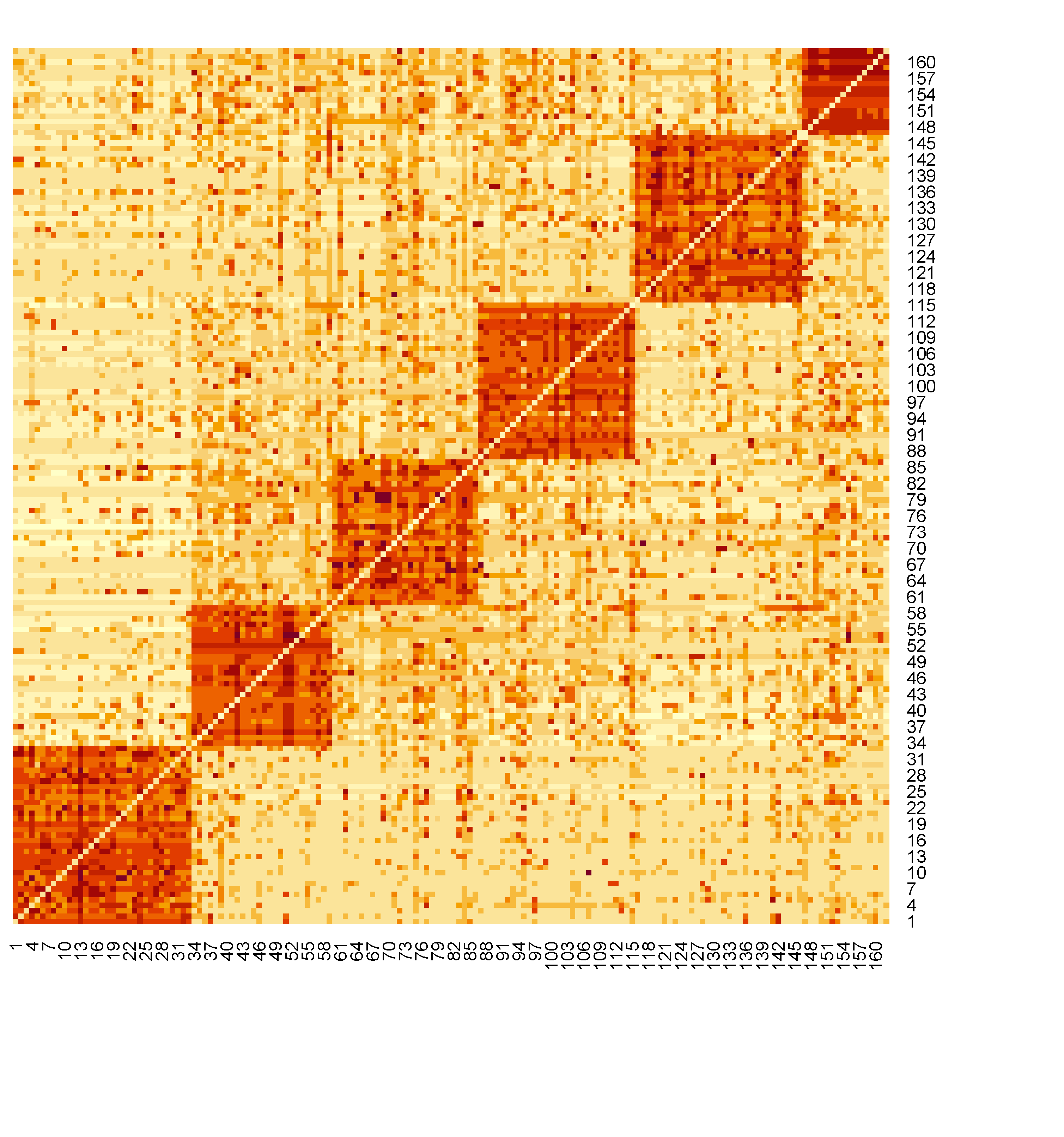
Figure 1: Heatmap of the friendship network. Darker color indicates a higher
level friendship
Keywords: Friendship network ● Personality ● Social network analysis ● Quadratic relation ● Factor analysis
Social relations play a crucial role in an individual’s social and behavioral development (Cacioppo & Cacioppo, 2014; House, Landis, & Umberson, 1988; McCamish-Svensson, Samuelsson, Hagberg, Svensson, & Dehlin, 1999; Umberson, Crosnoe, & Reczek, 2010). Close and healthy social relations benefit people’s subjective well-being in their life span (McCamish-Svensson et al., 1999; Seeman, 2001; Waldinger, Cohen, Schulz, & Crowell, 2015). Social relations also impact people’s health behavior such as alcohol use (Balsa, Homer, French, & Norton, 2011). Understanding and predicting the formation of social relations is thus of enormous interests to researchers and has been traditionally studied in social and personality psychology (e.g., Bahns, Crandall, Gillath, & Preacher, 2017; Cacioppo & Cacioppo, 2014)
In the existing literature, the principle of homophily is “believed” to be the mainstream of the formation of social relations. In other words, individuals in close social relations share many similar characteristics (McPherson, Smith-Lovin, & Cook, 2001; Rushton & Bons, 2005). A large body of research has investigated the presence of similar personality attributes in close relations such as romantic relations and friendships (e.g., Asendorpf & Wilpers, 1998; Harris & Vazire, 2016; Liu, Jin, & Zhang, 2018; Youyou, Stillwell, Schwartz, & Kosinski, 2017). Much of the research found no or weak personality similarity (Altmann, Sierau, & Roth, 2013; Watson, Beer, & McDade-Montez, 2014; Watson, Hubbard, & Wiese, 2000). Others found moderate similarities in some of the Big Five personality factors (McCrae et al., 2008). Youyou et al. (2017) revealed personality similarity among couples and friends. Another study found that individuals tended to select those with similar personalities as friends (Bahns et al., 2017). Hudson and Fraley (2014) found a quadratic relationship between partners’ personality-trait-similarity and relationship satisfaction among people with low avoidance and high anxiety. The existing conclusions seem to be inconclusive.
There are at least two potential reasons that account for the inconsistency in the literature. In most of these studies, only data on dyads are available due to the data collection methods such as collecting data from friends whereas data on dyads without social relations are not available. Therefore, few of these studies actually contrasted the two types of dyads due to the lack of the baseline group. Moreover, correlation analysis is the dominant approach used in studying the similarities of two actors forming dyads, which only focuses on the linear relationship between two variables and oversights the potential nonlinear relationships.
Social network data, however, contain both dyads with social relations and dyads without social ties. A social network comprises a group of actors and the potential relationship between them (Wasserman & Faust, 1994). In a network graph $\bf M$, nodes represent “actors,” and they could be any entities such as students in a friendship network, research institutions in a collaboration network, and variables in a variable network (Epskamp, Rhemtulla, & Borsboom, 2017). The ties/edges in a network display the relations, interactions or dependence among “actors.” It thus provides a premise to study the association between actor attribute similarity and social relations as in previous studies. It further allows researchers to compare two types of dyads using tools other than correlation analysis. It potentially leads to more interpretable results. In recent years, efforts have been made to address social and psychological research questions from the network perspective. Sweet (2016) reviewed common descriptive methods and network models for educational and psychological research. Clifton and Webster (2017) discussed the use of social network data to address psychological research questions through several examples. Liu et al. (2018) proposed a structural equation model to predict the existence of binary social relations using the latent personality distance.
The goal of the present work is multifold. First, we introduce some measures to quantify dyads’ properties, which are named “nodal/dyadic” covariates. These measures are not necessarily about similarity but could be in any meaningful format. Second, we demonstrate how to use the newly introduced measures to predict social relations using the proposed model by Liu et al. (2018), which provides a primer on predicting social bonds in a network. Third, we illustrate how to conduct the model selection and choose the model that fits the data best.
The rest of this article is structured as follows. First, we describe the college friendship network data collected by the Lab of Big Data at the University of Notre Dame. Next, we explore the factor structures of personality data. We then predict a valued friendship network using student’s characteristics and select the model that fits the data best. In the end, we conclude the study with discussions on the current development and future directions.
Throughout this paper, we use the data collected by the Lab of Big Data at the University of Notre Dame (Liu et al., 2018).
The participants are 162 students in a 4-year college in China. All the students were studying at the school of art and letters while completing the survey. Therefore, the boundary of the friendship network was known before data collection. Among the 162 students, there were 90 female and 72 male students. Their average age was 21.64 years (SD=0.86).
Four types of information are available: (1) friendship networks, (2) actor attributes including demographic information, (3) behaviors, and (4) personalities.
To collect the network data, we gave each student a roster of all the 162 students and asked them to report their acquaintanceship with every other student. The friendship was measured on a 5-point Likert scale ranging from “I have never heard about this student.” to “The person is one of my best friends.” (See Table 1).
| Level | Meaning
| |
| 0 | I have never heard the name. | |
| 1 | I heard about the person but had no personal interaction with her/him. | |
| 2 | I have met the person a few times but he/she is not a friend of mine. | |
| 3 | The person is a friend of mine. | |
| 4 | The person is one of my best friends. | |
In the current study, we used the maximal relationship between a pair of students. If two students have different evaluations on the friendship between them, we use the stronger evaluation. Therefore, the relationship is symmetric and non-directional. With 162 students, the network data are recorded in a 162 by 162 matrix $\bf M$, which is called a “sociomatrix” in the field of social network analysis. A row of $\bf M$ contains the responses of the row actor on their friendship relations with the column actors.
A plot of the friendship network with ordinal relations is included in Figure 1. In the heatmap of the friendship network, a darker square represents a stronger relationship between the students in the corresponding row and column. On the diagonal from the bottom left to the upright, there are six blocks standing out with dark color, each containing a group of students with closer relations. Those blocks are clusters of the college student friendship network.
We used the 20-item Mini-IPIP Scale for the Big Five factors of personality (Donnellan, Oswald, Baird, & Lucas, 2006). The five factors measured include Intellect/Imagination (or Openness), Conscientiousness, Extraversion, Agreeableness, and Neuroticism. Each of the five factors is measured by 4 items. Example items of the Mini-IPIP scale are: “In general, I am the life of the party” and “I am not interested in abstract ideas.” The 20 items were rated on a 5-point Likert scale (i.e., 1 = strongly disagree, 2 = somewhat disagree, 3 = neither agree nor disagree, 4 = somewhat agree, and 5 = strongly agree). For reverse coded items, the scores were reversed before analysis.
Participants also reported data on their behaviors. Participants rated themselves on these items using a true or false format. To collect data on the alcohol use, each student reported whether they had drunk alcohol in the past 30 days or not. Among the 162 students, 68 students reported they have drunk alcohol in the past thirty days. Besides, information on academic performance was also available, with scores ranging from 18 to 87. The average academic performance score was 54.99, with a standard deviation of 10.94.
The purpose of the analysis is to exemplify the potentials of social network analysis in psychological research. Specifically, we will investigate how personality predicts friendship. In the literature, there are arguments on both “Birds of a feather flock together,” and “Opposites attract.” If birds of a feather flock together, then we can expect that students with similar personality traits should be more likely to be friends. If opposites attract, then we can expect those with dissimilar personalities should boost the likelihood for them to be friends. If both statements are plausible, then we should expect a nonlinear relation between personality similarity and friendship. In the following, we will first explore the factor structures of personalities.
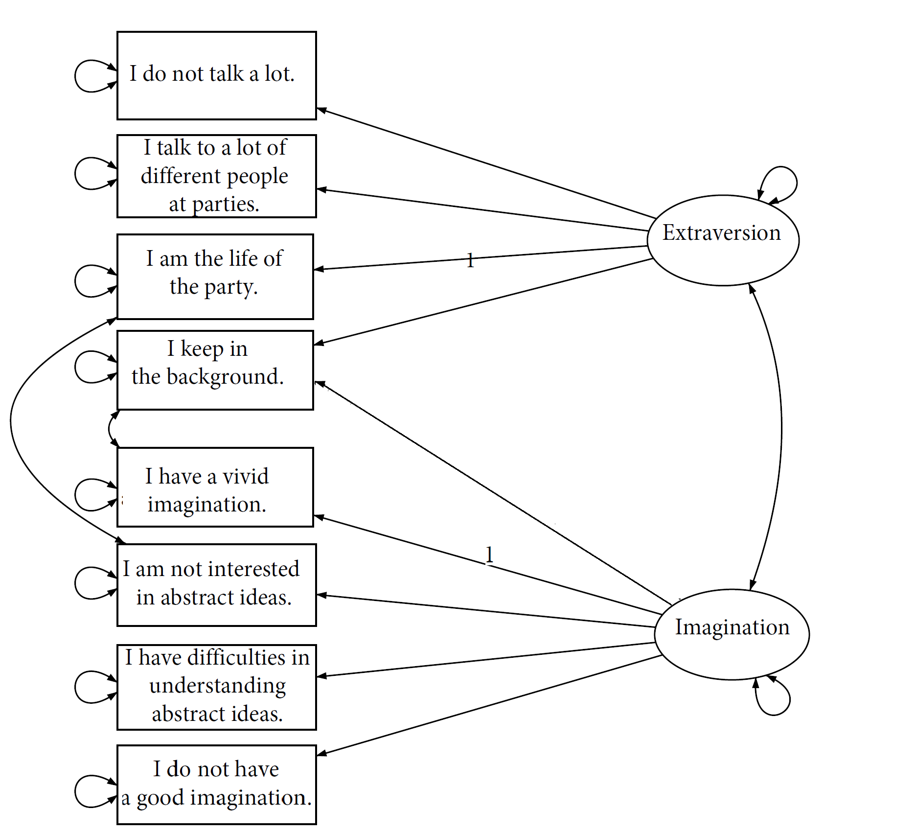
We conducted a confirmatory factor analysis (CFA, Cattell, 1952) to evaluate the structure of the latent personality traits. The reliability ($\alpha $) of the five scales are 0.57 for “intelligence/imagination”, 0.48 for “conscientiousness”, 0.62 for “extraversion”, 0.48 for “agreeableness”, and 0.40 for “neuroticism.” We decided to use two factors$-$imagination and extraversion$-$in the CFA because they have relatively high $\alpha $ values. Let $\boldsymbol {\eta }$ be the vector of latent personality factors and $\bf w$ be their indicators. The CFA model has the following general form,
 | (1) |
where ${\bf w}_{i}$ is the indicator data on actor $i$, $\boldsymbol {\varepsilon }_{i}$ is a $J\times 1$ vector of unique factors and it follows a multivariate normal distribution with mean $\boldsymbol {0}$ and covariance matrix $\bf \Psi $. The factor loading matrix $\mathbf {\Lambda }$ is a $J\times D$ matrix. $\bf \boldsymbol {\Phi }$ is the factor covariance matrix to be estimated. In this model, the unknowns include individuals’ factor scores $\{\boldsymbol {\eta }_{i}\}_{i=1}^{N}$ and model parameters $\{{\bf \Lambda },{\bf \boldsymbol {\Phi }},{\bf \Psi }\}$. We fix one factor loading of each factor to be 1 for the purpose of model identification.
We conducted model modification after fitting the model without cross-loadings and correlations among items to explore the factor structure. We ended up with the final model with RMSEA 0.047 and CFI 0.963. The path diagram of the final model is presented in Figure 2.
Recall that the purpose of the current study was to investigate the association between personality similarity and friendships. We, therefore, recorded estimates for both the factor covariance matrix $\bf {\Phi }$ and individuals’ factor scores $\boldsymbol {\eta }_i$, which will be used to compute the personality similarity (i.e., distance) of any two students. The estimated factor covariance matrix is provided in Table 2.The variance estimates of extraversion and imagination are 0.838 and 0.252, respectively, and their covariance is 0.172.
| cov(,) | Extraversion | Imagination |
| Extraversion | 0.838 | 0.172 |
| Imagination | 0.172 | 0.252 |
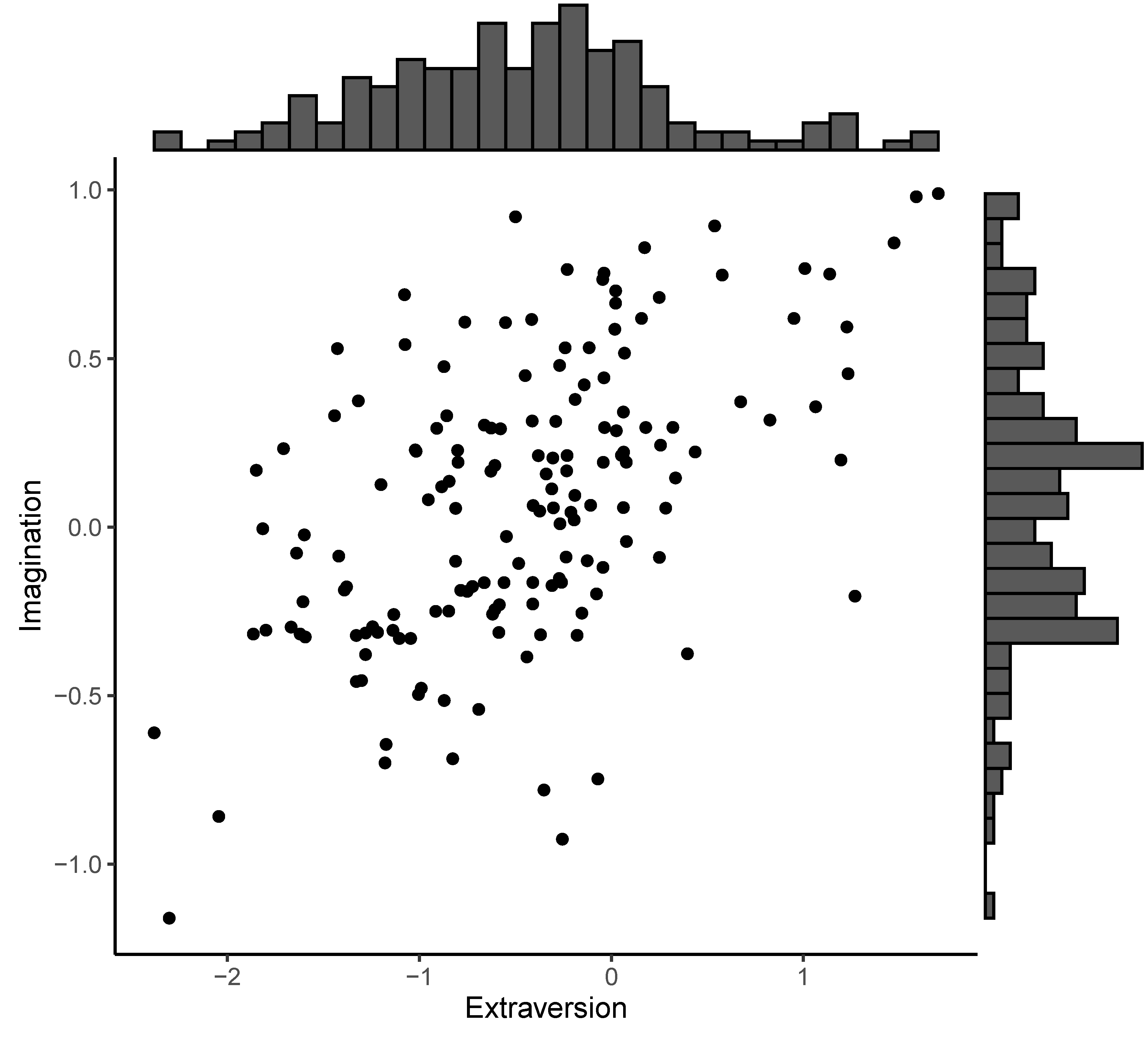
Despite many factor score estimators, the Thurstone-Thomson “regression” factor scores (Thurstone, 1935) were extracted and used in the subsequent analysis following the recommendations by both Devlieger, Mayer, and Rosseel (2016) and Liu et al. (2018). The scatterplot and the histograms of the predicted factor scores are provided in Figure 3. Each dot in Figure 3 represents the location of a student in the personality space formed by the scores of extraversion and imagination. Two students sharing similar personality traits in extraversion and imagination would stay close to each other in the personality space.
The model we will introduce is built on the prior work on structural equation modeling of social networks by Liu et al. (2018). In this modeling framework, individuals are assumed to hold a position in a latent space formed by personality traits (i.e., personality space). The distance/(dis)similarity between two individuals in the personality space predicts how likely they connect in the manifest social world. This modeling framework is developed to predict social relations using individuals’ characteristics. This model can particularly investigate whether similar personalities or dissimilar personalities boost friendships among college students.
In the following, we will present the model in a form for analyzing networks with ordinal relations and demonstrate its applications in examining the relationship between personality similarity and friendships. We will compare the following plausible hypotheses: (1) similar personality traits promote friendship; (2) dissimilar personality traits imply a higher chance to be friends; or (3) both are plausible.
The data analysis will use a three-phase procedure. First, we will define “nodal covariates” (i.e., dyads level covariates) based on the research hypotheses of interests. Second, we will build a Probit model to investigate how the nodal covariates predict friendship. Third, we will conduct likelihood ratio tests to select the model with the best fit for the data.
The study focuses on predicting the ordinal ties in the friendship network, which is a dyadic level analysis of social networks. Therefore, we need to construct dyadic covariates describing the characteristics of a pair of students. In addition to personality traits, we also consider three manifest covariates-gender, academic performance, and class membership.
Same-gender friendship has been of interest to researchers (Benenson, 1990; Elkins & Peterson, 1993; Jones, 1991; Zarbatany, Conley, & Pepper, 2004). To test the effect of gender on friendship, we define the following nodal covariate, \[ h_{\text {gender}}(i,j) =\begin {cases} 1 & \text {if students } i \text { and } j \text { are of the same gender}\\ 0 & \text {otherwise}. \end {cases} \] Using the nodal covariate $h_{\text {gender}}$, we can study the homogeneous gender effect on the acquaintance levels.
Academic achievement is measured using a continuous scale. To quantify the similarity in academic achievement, we define a nodal covariate of academic achievement as the absolute difference of two students’ scores \[ h_{\text {score}}(i,j)=|\text {score}_{i}-\text {score}_{j}|. \] The larger value on $h_{\text {score}}(i,j)$, the more discrepancy of students $i$ and $j$ on their academic achievement.
The 162 students participating in our study belonged to different “classes.” Students from the same class take the same courses more often, and potentially have more chances to build friendships. Therefore, we control the class membership effect in our analysis. The nodal covariate of class membership takes value one if two students are from the same class and 0 otherwise. That is \[ h_{\text {class}}(i,j)=\begin {cases} 1 & \text {if students } i \text { and } j \text { are from the same class,}\\ 0 & \text {otherwise}. \end {cases} \]
In addition to the three manifest nodal covariates $h_{gender}$, $h_{score}$, and $h_{class}$, we focus on the relationship between the personality similarity and friendships. To quantify the personality similarity, we use the Mahalanobis distance (Mahalanobis, 1936) of the personality factor scores of two students,
where $\boldsymbol {\eta }_{i}$ and $\boldsymbol {\eta }_{j}$ are the vectors of personality factor scores of students $i$ and $j$, and $\bf \Phi $ is the covariance matrix of personality latent factors. The Mahalanobis distance is the standardized distance of two correlated vectors penalized by the covariance between them.
We want to note that the concept of the “nodal” covariate is flexible to include any statistics that summarize the information of dyads. Researchers can define their nodal covariates based on their research hypothesis. Moreover, a nodal covariate is not necessarily capturing the similarity of actors as exemplified. Instead, it could be of any type. To provide an example, one can define overall academic achievement as the sum of scores of two students and test whether the overall score relates to the friendship or not. Instead of studying the effect of similar personality, one could also study the overall extraversion level of two students and investigate its impact on the friendship between the two students.
To model the association between personality similarity and friendship, we extended the work by Liu et al. (2018) to undirected valued networks with ordinal relations. A probit model is adopted to predict the ordinal relations using nodal covariates (Agresti, 2013). Let $m_{ij}$ be the level of friendship between student $i$ and $j$. It could take one of the five ordinal values 0, $1, 2, 3$, or $4$ in the college friendship introduced in the previous section. A greater value indicates a stronger relationship between the two students. For a level $k=0,1,2,\cdots ,4$, let $\pi _{ij}^{(k)}$ be the probability for $m_{ij}$ to be in the $k$’th category,
The cumulative probability for a tie in a category $k$ and below is
and $\sum _{k=0}^{4}\pi _{ij}^{(k)}=1$, since any friendship tie must fall in one of the five categories. To predict the probability for a tie to fall in a category using nodal statistics on dyads, we use an ordered probit model,
![(| Probit [p(m ≤ k)] = F- 1[p(m ≤ k)] for k = 0,1,⋅⋅⋅,3
{ ij ij′
|( (4) = τk|k+∑13 - (β h(ki)j + γdij)
πij = 1- k=0πij](v1n1p34x.svg)
| (5) |
where $F(\cdot )$ is the cumulative density function (CDF) of the standard normal distribution (i.e., N(0, 1)), and $d$ is the latent personality distance computed as $d=\sqrt {(\boldsymbol {\eta }_{i}-\boldsymbol {\eta }_{j})^{t}{\bf \Phi }^{-1}(\boldsymbol {\eta }_{i}-\boldsymbol {\eta }_{j})})$ as in Equation (2). The parameters $\boldsymbol {\beta }$ and $\gamma $ are coefficients of manifest nodal covariates and latent factor distance (i.e., $d$). Because $F^{-1}(\cdot )$ is an increasing function, the intercept coefficients must follow an ordered sequence, \[ \tau _{0|1}\leq \tau _{1|2}\leq \cdots \leq \tau _{3|4}. \]
To further understand the impact of the slope parameter $\gamma $ on the propensities of categories, four plots with different values for $\gamma $ are provided in Figure 4. We generate data from a model with four categories, and the three thresholds are $\tau _{0|1}=-1$, $\tau _{1|2}=0$, and $\tau _{2|3}=1$ and one manifest covariate (i.e., $h1$) whose coefficient $\beta =0.6$. Given $h1=0$, we computed the implied cumulative probabilities with varying $d$. In Figure 4, the red, green, blue, and purple curves are the probability for a tie in category 0, category 0 or 1, category 0, 1, or 2, and category 0, 1, 2, or 3.
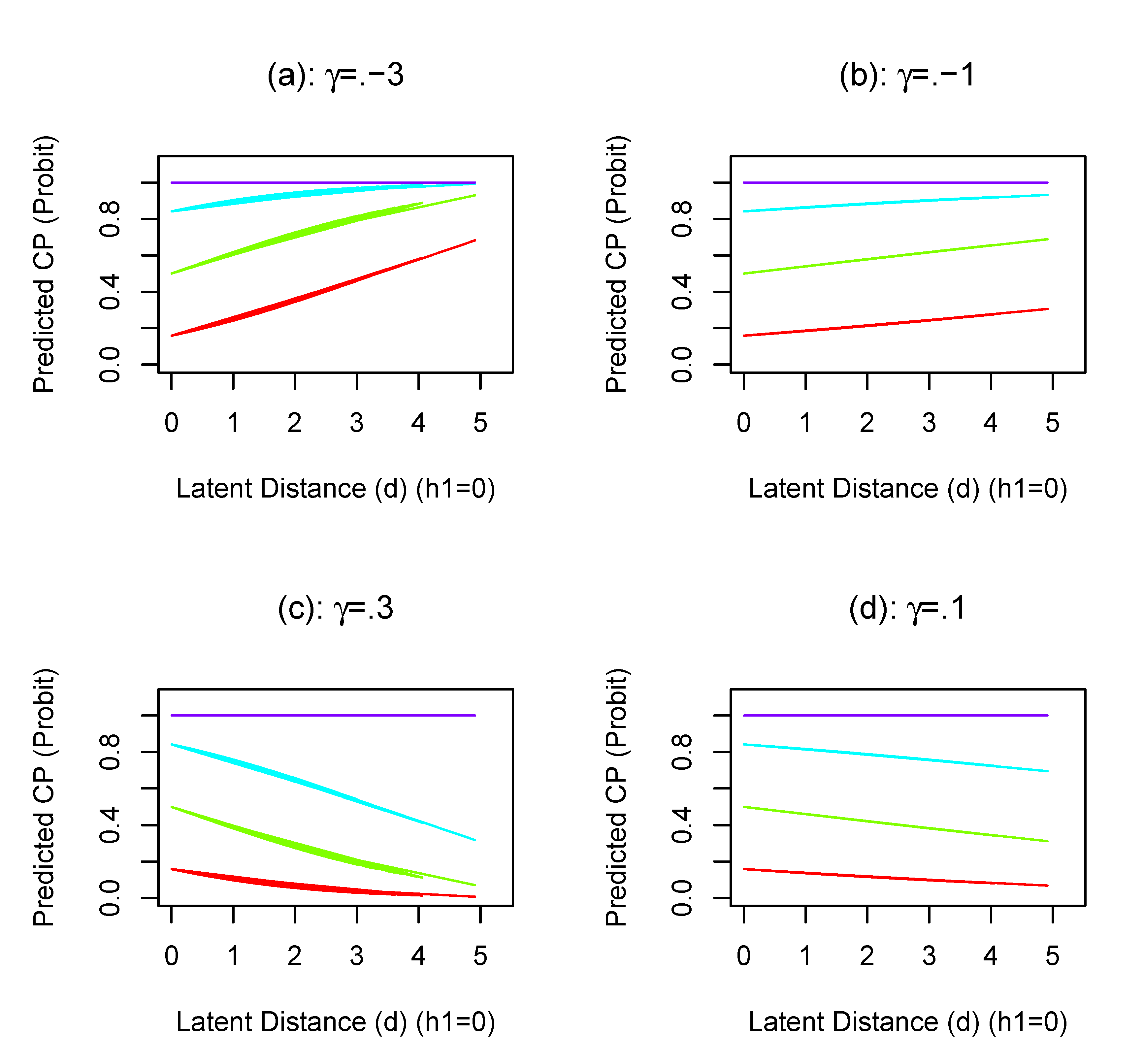
First, when $\gamma <0$ (Plot (a) and (b) in Figure 4), the cumulative probabilities are increasing as the latent distance $d$ increases. Thus, the probability for a tie in a higher-level category decreases. When $\gamma >0$ (Plot (c) and (d)), the trajectories of the cumulative probability are in the opposite direction. A positive value of $\gamma $ indicates that with a larger latent distance $d$, the probability for a relationship to be in a higher-level category increases. The magnitude of $\gamma $ (i.e., $|\gamma |$) tells the extent to which the latent distance affects the cumulative probability. A larger $|\gamma |$ implies stronger impacts of latent distance $d$ on the friendship.
To investigate the potential higher-order relationship between the personality similarity and friendship, we fit the model with the quadratic term of personality distance. To check whether the quadratic model is the conclusive model, we can fit the model with the cubic term of the personality distance. Therefore, we fit three competing models: a linear model with the first-order distance, i.e., $d_{ij}$ as a predictor, a quadratic model with $d_{ij}^{2}$ as a predictor, and a cubic model with $d_{ij}^{3}$ as a predictor.
In the linear probit model, we include three manifest nodal covariates $h_{gender},h_{score}$, and $h_{class}$ as well as the latent personality distance $d$,
![(
||P (mij ≤ k) = π0ij + π1ij + ⋅⋅⋅+ π(ijk), for k = 0,1,⋅⋅⋅,4.
||||Probit [P(mij ≤ k)] = F-1[P(mij ≤ k)] for k = 0,1,⋅⋅⋅,3
{
|| = τk|k+1 - (β1hgender(i,j)+ β2hscore(i,j)
|||| +β3hcla∑ss(i,j)+ γdij)
(π(i4j) = 1- 3k=0π(ikj)](v1n1p35x.svg)
| (6) |
In this model, the coefficient $\gamma $ explains the extent to which the personality distance $d_{ij}$ predicts friendship. With a negative $\gamma $, the probability of having a higher level of friendship is greater when $d_{ij}$ is smaller, so the more similar personalities associate with a higher chance to have a closer friendship. If $\gamma $ is positive, then dissimilar personalities boost friendship.
In the second model, we also include a quadratic term of the latent personality distance, and the model becomes,
This model is useful for investigating the potential quadratic relationship between the personality similarity and friendship, and it also helps identify the transition points of the trend.
The cubic model includes the third-order of the distance, i.e., $d_{ij}^{3}$, in the analysis,
By fitting the cubic model, we can investigate if there is more than one transition point for the relationship between personality similarity and friendship.
To estimate the model, we first evaluate the factor structure of the extroversion and imagination, and obtain the model parameter estimates and the Thurstone-Thomson “regression” factor scores $\hat {\boldsymbol {\eta }_{i}}$ and $\hat {\boldsymbol {\eta }_{j}}$ as discussed in the previous section. We then compute the estimated personality distance \[ \hat {d}_{ij}=\sqrt {(\hat {\boldsymbol {\eta }}_{i}-\hat {\boldsymbol {\eta }}_{j})^{t}\hat {\bf {\Phi }}^{-1}(\hat {\boldsymbol {\eta }}_{i}-\hat {\boldsymbol {\eta }}_{j})}. \] According to the suggestions by Liu et al. (2018), the use of Thurstone-Thomson factor scores led to asymptotically unbiased estimates for the $\gamma $ parameter.
In this section, we will present the results of the three models discussed in the previous section
To evaluate the relative performance of the three models (i.e., linear, quadratic, and cubic probit model), we conducted likelihood ratio tests using the saved deviance in Table 3. For the linear model against the quadratic model, the Chi-square statistic is 9.514 and with a p-value of .002. Hence, the quadratic model is significantly better than the linear model. When the quadratic model is compared against the cubic (third-order) model, the Chi-square statistic is 0.318 with a p-value of .573. Thus, the cubic model is not significantly better than the quadratic model. The quadratic model is thus the best model.
| Model | Deviance | Test | Df | LR Stat | Pr(Chi) | ||
| 1 | Linear | 28560.55 | |||||
| 2 | Quadratic | 28551.03 | 1 vs 2 | 1 | 9.514 | .002 | |
| 3 | Cubic | 28550.71 | 2 vs 3 | 1 | 0.318 | .573 | |
Because the quadratic model fits the data best, we would interpret the relationship between the personality similarity and friendship using the estimates of the quadratic model, which are provided in Table 4.
| Par | Est | Std.Error | t.value | p-value | |
| $\beta _{\mbox {gender}}$ | 0.549 | 0.02 | 26.839 | $<.001$ | |
| $\beta _{\mbox {score}}$ | -0.111 | 0.013 | -8.773 | $<.001$ | |
| $\beta _{\mbox {class}}$ | 2.439 | 0.032 | 75.549 | $<.001$ | |
| $\gamma _{1}$ | -0.098 | 0.044 | -2.238 | .025 | |
| $\gamma _{2}$ | 0.038 | 0.012 | 3.088 | .004 | |
| $\tau _{0}$ | 0.228 | 0.04 | 5.694 | $<.001$ | |
| $\tau _{1}$ | 1.113 | 0.041 | 27.214 | $<.001$ | |
| $\tau _{2}$ | 1.720 | 0.043 | 40.097 | $<.001$ | |
| $\tau _{3}$ | 2.888 | 0.049 | 58.565 | $<.001$ | |
| Residual deviance | 228551.03
| ||||
By plugging the model parameter estimates into the quadratic model (Equation 7), we obtained the predicted cumulative probability for a tie to be in a category $k$ ($k$=0,1,2 or 3) or below1. Equivalently, we can also get the probability for a tie to be in a category above $k$( $k=0,1,2$, or $3$)2 and we will use them for the interpretation in the following.
First, all parameters are statistically significant, based on the significance level of 0.05. The coefficient of $h_{gender}$ is 0.549. Given the levels for other covariates and latent personality distance being the same, two students of the same gender tend to have a closer relationship than otherwise, and they are less likely to have a lower-level friendship. Therefore, gender homogeneity boosts a higher level of acquaintanceship. Second, the coefficient $h_{score}$ has a point estimate -0.111 (p-value$<0.001$). Given the same levels of other covariates and latent distance, students with more similar academic achievement (i.e., $h_{score}$ is small) have a higher level of friendship with a greater probability than two students with some very different academic achievements. Third, the coefficient estimate of $h_{class}$ is 2.439. Thus, two students from the same class are more likely to have a closer relationship. For instance, $\pi ^{(4)}$ is larger for two students from the same class.
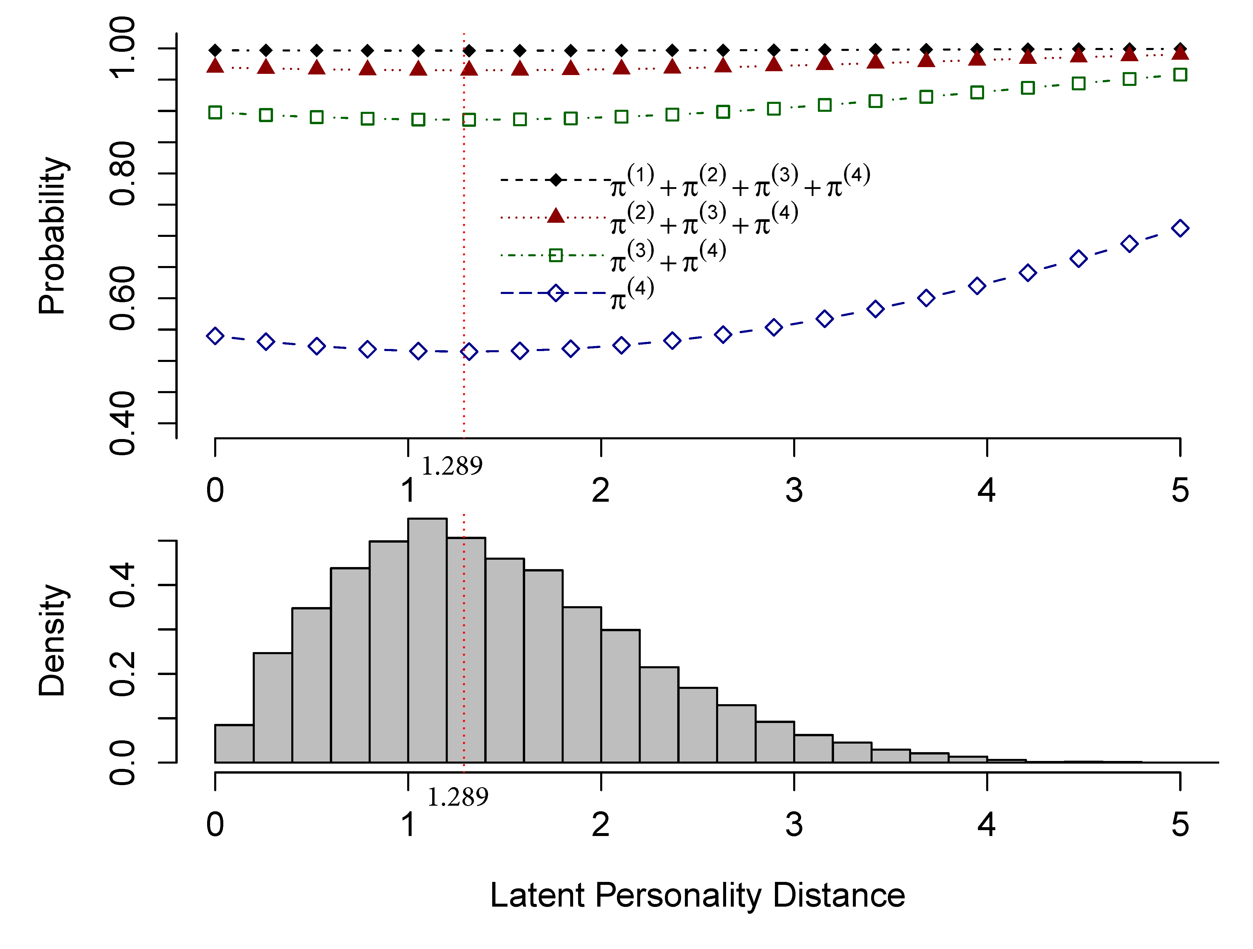
The coefficient estimate of the first-order distance (i.e., $\gamma _{1}$) is -0.098 (p-value =0.025) and that of the second-order distance is 0.038 (p-value= .004). For $k=0,1,2,\text {or }3$, the quantity $\pi ^{(k+1)}+\cdots +\pi ^{(4)}$ is the probability for a tie to fall in a category above $k$. To better understand the relationship between personality similarity and friendship, we plotted these probabilities against the latent personality distance $d$, given two students are of the same gender (i.e., $h_{gender}=1$), have the same academic score (i.e., $h_{score}=0$), and are from the same class (i.e., $h_{class}=1$). These plots are provided in Figure 5.
All four probability curves are U-shapes. They decrease first and increase afterward when the latent distance increases. They reach their minimum values when the latent personality distance between the two students is 1.289. When the latent distance approaches 0, the probability for a tie in a category above $k$ (for $k=0,1,2$, or $3$) becomes larger, which indicates that the propensity for two students to have a higher level of acquaintanceship increases. Thus, similar personalities in extraversion and imagination are beneficial to the friendship between two students. When the latent personality distance is greater than 1.289, the probability for a friendship to be in a category above $k$ increases with a larger latent personality distance. Thus, dissimilar personalities in extraversion and imagination also contribute to friendship. The results from this empirical study clearly support both “Birds of a feather flock together,” and “Opposites attract.”
Social network analysis has been increasingly popular in recent decades. Network data are now easy to collect than ever due to the development of computer techniques. A social network comprises two primary elements: actors and potential social ties. There are observations on both dyads with social relations and dyads without social relations in social network data. Therefore, it allows researchers to understand what and how actors’ characteristics predict social relations by contrasting these two groups of dyads. In the current study, we illustrated how to predict social relations using actors’ characteristics by analyzing a college friendship network.
To analyze the ordinal/valued friendship network, we extended the work by Liu et al. (2018), which was built to analyze social networks with binary relations. A probit regression model was used to predict the ordinal social ties using the information of dyads. Specifically, we studied how gender homogeneity, similar academic achievements, class membership, and similar personalities predicted college student’s friendship. To investigate the potential quadratic relationship between personality similarity and friendship, we fitted three competing models: a linear model with only the linear term of latent distance (i.e., $d$), a quadratic model with both a linear term and a quadratic term of the latent personality distance (i.e., both $d$ and $d^{2}$), and a cubic model with also the third order of the latent personality distance. The quadratic model was significantly better than the linear model but not statistically different from the cubic model. Therefore, the quadratic models won both the linear and cubic models.
Based on the results of the quadratic model, students of the same gender or from the same class were more likely to have closer friendships. Students with similar academic scores were more likely to have higher levels of acquaintanceship. The association between personalities and friendship was mixing. Two students tended to have closer friendship relations if they had very similar personalities in extroversion and imagination. At the same time, if they were very dissimilar in those two personality traits, their friendship was more likely to fall in a higher level category. Hence, “Both birds of a feather flock together” and “Opposites attract” are possible.
Although we fitted the model for undirected networks, the modeling framework could be extended for networks with directed relations. Based on the heatmap (Figure 1), there are several communities/clusters in the college friendship network. In a cluster, students share some common characteristics. In the future, we would also like to fit multilevel models for the potential heterogeneity in the relationship between personality and friendship.
This study is partly supported by a grant from the Department of Education (R305D210023). However, the contents of the study do not necessarily represent the policy of the Department of Education, and you should not assume endorsement by the Federal Government. We thank the reviewer and the guest editor for their instructive comments and suggestions.
Agresti, A. (2013). Categorical data analysis (3rd ed.; D. J. Balding, N. A. Cressi, G. M. Fitzmaurice, H. Goldstein, & I. M. Johnstone, Eds.). Hoboken, N.J.: John Wiley & Sons, Inc..
Altmann, T., Sierau, S., & Roth, M. (2013). I guess you’re just not my type: Personality types and similarity between types as predictors of satisfaction in intimate couples. Journal of Individual Differences, 34(2), 105–117. doi: https://doi.org/10.1027/1614-0001/a000105
Asendorpf, J. B., & Wilpers, S. (1998). Personality effects on social relationships. Journal of Personality and Social Psychology, 74(6), 1531–1544. doi: https://doi.org/10.1037/0022-3514.74.6.1531
Bahns, A. J., Crandall, C. S., Gillath, O., & Preacher, K. J. (2017). Similarity in relationships as niche construction: Choice, stability, and influence within dyads in a free choice environment. Journal of Personality and Social Psychology, 112(2), 329–355. doi: https://doi.org/10.1037/pspp0000088
Balsa, A. I., Homer, J. F., French, M. T., & Norton, E. C. (2011). Alcohol use and popularity: Social payoffs from conforming to peers’ behavior. Journal of Research on Adolescence, 21(3), 559–568. doi: https://doi.org/10.1111/j.1532-7795.2010.00704.x
Benenson, J. F. (1990). Gender differences in social networks. The Journal of Early Adolescence, 10(4), 472–495. doi: https://doi.org/10.1177/0272431690104004
Cacioppo, J. T., & Cacioppo, S. (2014). Social relationships and health: The toxic effects of perceived social isolation. Social and personality psychology compass, 8(2), 58–72. doi: https://doi.org/10.1111/spc3.12087
Cattell, R. B. (1952). Factor analysis: an introduction and manual for the psychologist and social scientist. Harper.
Clifton, A., & Webster, G. D. (2017). An introduction to social network analysis for personality and social psychologists. Social Psychological and Personality Science, 8(4), 442–453. doi: https://doi.org/10.1177/1948550617709114
Devlieger, I., Mayer, A., & Rosseel, Y. (2016). Hypothesis testing using factor score regression: A comparison of four methods. Educational and Psychological Measurement, 76(5), 741–770. doi: https://doi.org/10.1177/0013164415607618
Donnellan, M. B., Oswald, F. L., Baird, B. M., & Lucas, R. E. (2006). The mini-ipip scales: Tiny-yet-effective measures of the big five factors of personality. Psychological assessment, 18(2), 192–203. doi: https://doi.org/10.1037/1040-3590.18.2.192
Elkins, L. E., & Peterson, C. (1993). Gender differences in best friendships. Sex Roles, 29, 497–508. doi: https://doi.org/10.1007/BF00289323
Epskamp, S., Rhemtulla, M., & Borsboom, D. (2017). Generalized network pschometrics: Combining network and latent variable models. Psychometrika, 82(4), 904–927. doi: https://doi.org/10.1007/s11336-017-9557-x
Harris, K., & Vazire, S. (2016). On friendship development and the big five personality traits. Social and Personality Psychology Compass, 10(11), 647-667. doi: https://doi.org/10.1111/spc3.12287
House, J. S., Landis, K. R., & Umberson, D. (1988). Social relationships and health. Science, 241(4865), 540–545. doi: https://doi.org/10.1126/science.3399889
Hudson, N. W., & Fraley, R. C. (2014). Partner similarity matters for the insecure: Attachment orientations moderate the association between similarity in partners’ personality traits and relationship satisfaction. Journal of Research in Personality, 53, 112–123. doi: https://doi.org/10.1016/j.jrp.2014.09.004
Jones, D. C. (1991). Friendship satisfaction and gender: An examination of sex differences in contributors to friendship satisfaction. Journal of Social and Personal Relationships, 8(2), 167–185. doi: https://doi.org/10.1177/0265407591082002
Liu, H., Jin, I. H., & Zhang, Z. (2018). Structural equation modeling of social networks: Specification, estimation, and application. Multivariate Behavioral Research, 53(5), 714–730. doi: https://doi.org/10.1080/00273171.2018.1479629
Mahalanobis, P. C. (1936). On the generalized distance in statistics. Proceedings of the National Institute of Sciences (Calcutta), 2, 49–55.
McCamish-Svensson, C., Samuelsson, G., Hagberg, B., Svensson, T., & Dehlin, O. (1999). Social relationships and health as predictors of life satisfaction in advanced old age: results from a swedish longitudinal study. The International Journal of Aging and Human Development, 48(4), 301–324. doi: https://doi.org/10.2190/GX0K-565H-08FB-XF5G
McCrae, R. R., Martin, T. A., Hrebickova, M., Urbánek, T., Boomsma, D. I., Willemsen, G., & Costa, P. T. (2008). Personality trait similarity between spouses in four cultures. Journal of personality, 76(5), 1137–1164. doi: https://doi.org/10.1111/j.1467-6494.2008.00517.x
McPherson, M., Smith-Lovin, L., & Cook, J. M. (2001). Birds of a feather: Homophily in social networks. Annual Review of Sociology, 27, 415-444. doi: https://doi.org/10.1146/annurev.soc.27.1.415
Rushton, J. P., & Bons, T. A. (2005). Mate choice and friendship in twins: evidence for genetic similarity. Psychological Science, 16(7), 555–559. doi: https://doi.org/10.1111/j.0956-7976.2005.01574.x
Seeman, T. (2001). How do others get under our skin ? Social relationships and health. In C.D.Ryff & B.H.Singer (Eds.), (pp. 189–210). Oxford University Press. doi: https://doi.org/10.1093/acprof:oso/9780195145410.003.0006
Sweet, T. (2016). Social network methods for the educational and psychological sciences. Educational Psychologist, 51(3-4), 381–394. doi: https://doi.org/10.1080/00461520.2016.1208093
Thurstone, L. L. (1935). The vectors of mind: Multiple-factor analysis for the isolation of primary traits. University of Chicago Press.
Umberson, D., Crosnoe, R., & Reczek, C. (2010). Social relationships and health behavior across the life course. Annual Review of Sociology, 36, 139–157. doi: https://doi.org/10.1146/annurev-soc-070308-120011
Waldinger, R. J., Cohen, S., Schulz, M. S., & Crowell, J. A. (2015). Security of attachment to spouses in late life: Concurrent and prospective links with cognitive and emotional well-being. Clinical Psychological Science, 3(4), 516–529. doi: https://doi.org/10.1177/2167702614541261
Wasserman, S., & Faust, K. (1994). Social network analysis: Methods and applications (Vol. 8). Cambridge university press.
Watson, D., Beer, A., & McDade-Montez, E. (2014). The role of active assortment in spousal similarity. Journal of Personality, 82(2), 116–129. doi: https://doi.org/10.1111/jopy.12039
Watson, D., Hubbard, B., & Wiese, D. (2000). Self–other agreement in personality and affectivity: The role of acquaintanceship, trait visibility, and assumed similarity. Journal of personality and social psychology, 78(3), 546–558. doi: https://doi.org/10.1037/0022-3514.78.3.546
Youyou, W., Stillwell, D., Schwartz, H. A., & Kosinski, M. (2017). Corrigendum: Birds of a feather do flock together: Behavior-based personality-assessment method reveals personality similarity among couples and friends. Psychological Science, 28(3), 276-284. doi: https://doi.org/10.1177/0956797616678187
Zarbatany, L., Conley, R., & Pepper, S. (2004). Personality and gender differences in friendship needs and experiences in preadolescence and young adulthood. International Journal of Behavioral Development, 28(4), 299–310. doi: https://doi.org/10.1080/01650250344000514
1 The predicted cumulative probability is computed as

2 The probability for a time to be in a category above $k$ ( $k=0,1,2$, or $3$)

For a level $k=0,1,2,$ or 3, the probability for tie to have a level above $k$ is analogous to the probability of being “1” if we dichotomize the ordinal relations into binary relations at the level $k$.