Figure 1: Imputation and analysis phase of the modified multiple imputation
approach for DTs.
Keywords: Multiple Imputation ● Classification and Regression Tree (CART) ● Missing Data
Missing data are endemic in research and appropriate handling of missing data is required to ensure unbiased parameter estimates. Missing data are often caused by participant nonresponse due to an unwillingness to divulge information, inadvertent skipping, fatigue, or time considerations (Hattie, 1983; Holman & Glas, 2005; Huggins-Manley, Algina, & Zhou, 2018; Moustaki & Knott, 2000). Missing data are particularly problematic when nonresponding participants systematically differ from participants who completed the study. Known as nonresponse bias (Lavrakas, 2008), systematic differences in responding may affect estimated model parameters and threaten the validity of conclusions drawn from the statistical model (Enders, 2010; Groves & Peytcheva, 2008; Lavrakas, 2008).
Several methods have been developed for handling missing data due to nonresponse (Baraldi & Enders, 2010). One widely recommended approach for handling missing data is multiple imputation (Allison, 2002; Baraldi & Enders, 2010; Enders, Dietz, Montague, & Dixon, 2006; Schafer & Olsen, 1998). Multiple imputation is a four-step procedure. First, plausible values from a distribution specifically modeled for the missing data are drawn. Second, the statistical model is fit to the imputed dataset and parameter estimates and standard errors are retained. Third, the first two steps are repeated a specified (e.g., 20) number of times. Fourth, the parameter estimates and standard errors are pooled to determine the point estimate for each parameter along with an appropriate standard error (Enders, 2010; Rubin, 1987; van Buuren & Groothuis-Oudshoorn, 2011). Proper standard errors are calculated to account for the within (square of the average standard error) and between (variance of the parameter estimates across imputations) imputation variation in the parameter estimates. This final step is referred to as the pooling step.
Multiple imputation is an effective missing data strategy for theoretically-driven statistical models (e.g., regression, ANOVA, etc.; Baraldi & Enders, 2010); however, the pooling step can be challenging when fitting exploratory/data driven models because the statistical models for each imputed dataset may include different model parameters (i.e., due to variable selection). Decision trees (DTs) are an exploratory model where the standard multiple imputation approach is not viable. In DTs, the data are recursively split into two nodes based on the variable and value that lead to an optimal prediction. Implementing the standard multiple imputation approach with DTs will likely lead to different variables being selected to partition the data in each imputed dataset, which makes the pooling stage challenging, if not impossible. In this paper, we propose and examine the performance of a modified multiple imputation approach for handling missing data with DTs. We compare the performance of the proposed approach against the standard approach for handling missing data in DTs (surrogate splits), simple missing data approaches (listwise deletion, delete if selected, and majority rule), single imputation, and a multiple imputation approach that ignores variation DT structures and pools the predicted values from the DTs (multiple imputation with prediction averaging). We continue with an overview of the classification and regression tree (CART) algorithm for DTs, review currently implemented missing data approaches in CART, and describe our proposed multiple imputation approach. We then outline and review our simulation study to evaluate the performance of each missing data approach, and conclude with recommendations.
CART is an algorithm for DTs that has become a very popular machine learning technique because of its ability to create powerful prediction models with nonlinear and interactive effects. Moreover, the resulting DT is easy to interpret. CART is a greedy DT algorithm that recursively partitions the data and considers the mean (quantitative outcome) or the mode (categorical outcome) as the predicted value within each partition (James, Witten, Hastie, & Tibshirani, 2013; Loh, 2011). Three critical aspects of the CART algorithm are variable splitting (fit criteria), stopping criteria, and model selection. For variable splitting, the CART algorithm selects the variable and partitioning value that splits the data into two groups where the outcome is maximally homogenous within each group (Breiman, Friedman, Stone, & Olshen, 1984). The two resulting groups are often referred to as child nodes (with the node that was split referred to as the parent node). All values of the predictors are considered potential splitting values to partition the data into two child nodes. For a regression tree (numeric outcome), the predictor variable and splitting value that minimizes the residual sum of squares is selected to split the node (Gonzalez, O’Rourke, Wurpts, & Grimm, 2018; Loh, 2011). For a classification tree (categorical outcome), the predictor variable and splitting value that minimizes the Gini Index (entropy/information can be used instead of the Gini Index) is selected to partition the node. This process in repeated on each child node until a stopping criterion is reached. Stopping criteria include a minimum improvement in prediction accuracy, tree depth, and sample size required to partition a node. These stopping criteria prevent further node splits, but are not often used for model selection. Once a stopping rule is reached for each node and tree growth has stopped, the DT is then pruned (reduced in size) with the final model selected based on k-fold cross-validation. A large DT is often grown in order to ensure that a useful split is not inadvertently missed because of an arbitrary stopping rule (Breiman et al., 1984).
Missing data occur when an observation contains no value for a given variable. There are numerous situations that lead to missing data, which makes it difficult to know exactly how and why each missing value appears in a dataset. Rubin (1976) proposed using observed variables to predict the occurrence of missing values and coined the term missing data mechanisms to classify relationships between missing values and the observed variables in a dataset. Specifically, missing data mechanisms describe how the propensity for a missing value relates to other measured variables and itself. Rubin (1976) presented three types of missing data mechanisms: missing completely at random (MCAR), missing at random (MAR), and missing not at random (MNAR). Data are MCAR when missing values on variable $x$ are unrelated to both the observed variables and the underlying values of $x$ itself (Enders, 2003; Rubin, 1976). Thus, MCAR indicates the occurrence of missing data is purely random making MCAR desirable; however, MCAR assumptions are rarely met in practice (Enders, 2010; Muthén, Kaplan, & Hollis, 1987; Raghunathan, 2004). Data are MAR when missingness is systematic and correlated with other variables in the dataset. Specifically, data are considered MAR when the missing values on the variable $x$ are related to other variables in a dataset but not related to $x$ itself (Enders, 2003; Rubin, 1976). Most advanced missing data handling procedures (e.g., multiple imputation, full information maximum likelihood) rely on MAR assumptions. Data are MNAR when missing values on $x$ are dependent on the underlying values of $x$ itself (Enders, 2003; Rubin, 1976). Missingness does not depend only on observed data when data are MNAR making it the most challenging missing data mechanism to handle in practice.
The missing data mechanisms determine how well a given missing data approach will perform. According to Baraldi and Enders (2010), deletion approaches (i.e., listwise, pairwise, etc.) perform well in situations when data are MCAR, whereas more advanced approaches, such as multiple imputation or full information maximum likelihood (FIML), outperform deletion and produce unbiased parameter estimates when data are MCAR or MAR. It is important to note that many approaches commonly used to treat missing data (e.g., deletion, imputation, FIML etc.) do not perform well when data are MNAR.
Missing data are problematic in CART because an observation with a missing value on the predictor variable provides no information about the child node to which the observation belongs. The advanced missing data techniques for handling MAR data, such as multiple imputation and full information maximum likelihood, cannot be applied in a straightforward manner in CART, and DTs more generally. Given the challenges for advanced missing data approaches, simpler strategies have been utilized in CART. We review these approaches next.
A simple missing data strategy for CART is to remove observations where a missing value is present. This approach is taken when preparing the data for analysis.
The second missing data strategy for CART is to retain participants with missing values until a variable with missing values is selected. For example, a participant has a missing value on $x_{1}$. This participant would be retained in the DT until $x_{1}$ is selected to partition the data. Thus, if $x_{1}$ is not selected, then the participant is retained in the model. Importantly, the participant contributes to the formation of the DT until s/he cannot be placed into a child node because of the missing value.
In majority rule, if a variable is selected for partitioning and a participant has a missing value, then the participant is placed in the child node that contains the most observations. Thus, the participant contributes to the formation of the DT even after the participant has a missing value for a selected splitting variable.
When an observation has a missing value on a selected splitting variable, surrogate splits uses another variable in the dataset to place the observation into a child node. That is, a surrogate variable is used to determine the child node for the observation with a missing value. To do this, the partitioning algorithm is applied with the two child nodes as a classification outcome and the other variables in the dataset as splitting variables (Therneau & Atkinson, 2019). The usefulness of each surrogate variable is determined by examining the misclassification error for each variable (misclassification error for predicting child node using participants with available data). Additionally, the misclassification rate is computed for majority rule, where observations with missing values on the splitting variable is placed in the child node with the most observations. Each variable that performs better than majority rule is considered a surrogate and is ranked based on its performance. The first-ranked surrogate variable is then used to place observations with missing values. If an observation is missing the first-ranked surrogate, then the second-ranked surrogate variable is used to place the observation, and so forth. In the rare situations where no surrogate variables are present, the observation is placed in whichever child node contains the most observations (Therneau & Atkinson, 2019).
Imputation strategies use information from the complete data to estimate what a missing value would be if it was observed. Single imputation draws a plausible value from a predictive distribution based on available data (Little & Rubin, 2002) to fill in a given missing value. The imputation model is typically built on a linear or logistic regression model depending on the nature of the variable with the missing values; however, imputation models have been built upon more complex algorithms, such as DTs and random forests (Tang & Ishwaran, 2017). Once data are imputed, the CART algorithm can be implemented using the imputed dataset, which does not have any missing values.
Multiple imputation with prediction averaging (Feelders, 1999; Twala, 2009) follows a fairly straightforward multiple imputation approach involving the four steps described above. First, missing values are imputed from a distribution specifically modeled for the missing data. Second, a DT is fit to the imputed data. Third, the first and second steps are repeated multiple (e.g., 20) times. Fourth, the predicted values from the DTs for an individual are averaged and the average serves as the predicted value for the individual. This approach does not try to summarize the decision rules of the DTs – just their predicted values. Thus, there is not a single DT with a single set of decision rules that can be interpreted. Averaging predicted values from the DTs fit to multiple imputed datasets is a viable approach when researchers are primarily interested in prediction because of the lack of interpretability. This approach will likely lead to better prediction accuracy because it is similar to bagging (Breiman, 1996).
Several studies have been conducted to compare DT missing data approaches (Batista & Monard, 2003; Beaulac & Rosenthal, 2020; Feelders, 1999; Twala, 2009). Across four studies, the following missing data approaches have been evaluated: listwise deletion, surrogate splits, single imputation (i.e., k-nearest neighbor imputation, mean/mode imputation, EM/logistic imputation, decision tree imputation, and distribution based imputation), multiple imputation with prediction averaging, separate class, Branch-Exclusive Splits Tree (BEST) algorithm, and several methods that were developed and implemented in other DT algorithms (e.g., C4.5 and C5.0). Nearly all studies used complete data sets (from the UCI machine learning repository) and artificially imposed missing values.
The studies that evaluated multiple imputation with prediction averaging found this approach outperformed all approaches it was compared against (e.g., single imputation, surrogate splits, listwise deletion) when data were MCAR and MAR (Feelders, 1999; Twala, 2009). The same studies found single imputation to be the second-best performing approach (Feelders, 1999; Twala, 2009). However, it is important to consider the different single imputation techniques. For example, EM single imputation performed well for numeric variables (Twala, 2009), whereas decision tree single imputation and k-nearest neighbor imputation performed best with categorical variables (Batista & Monard, 2003; Twala, 2009). Surrogate splits performed well when there are high correlations among variables (Twala, 2009) and listwise deletion generally performed poorly (Twala, 2009). Separate class and the BEST algorithm approaches have been found to perform well when data were MNAR (Beaulac & Rosenthal, 2020).
Previous research supports the current method of employing multiple imputation in DTs (i.e., averaging predicted values over different imputed tree structures) when data are MAR or MCAR, but only when a researcher is interested in prediction accuracy and not interested in interpretability. The purpose of this study is to modify the current multiple imputation approach in such a way that the proposed approach produces interpretable tree structures and reduces prediction accuracy inflation.
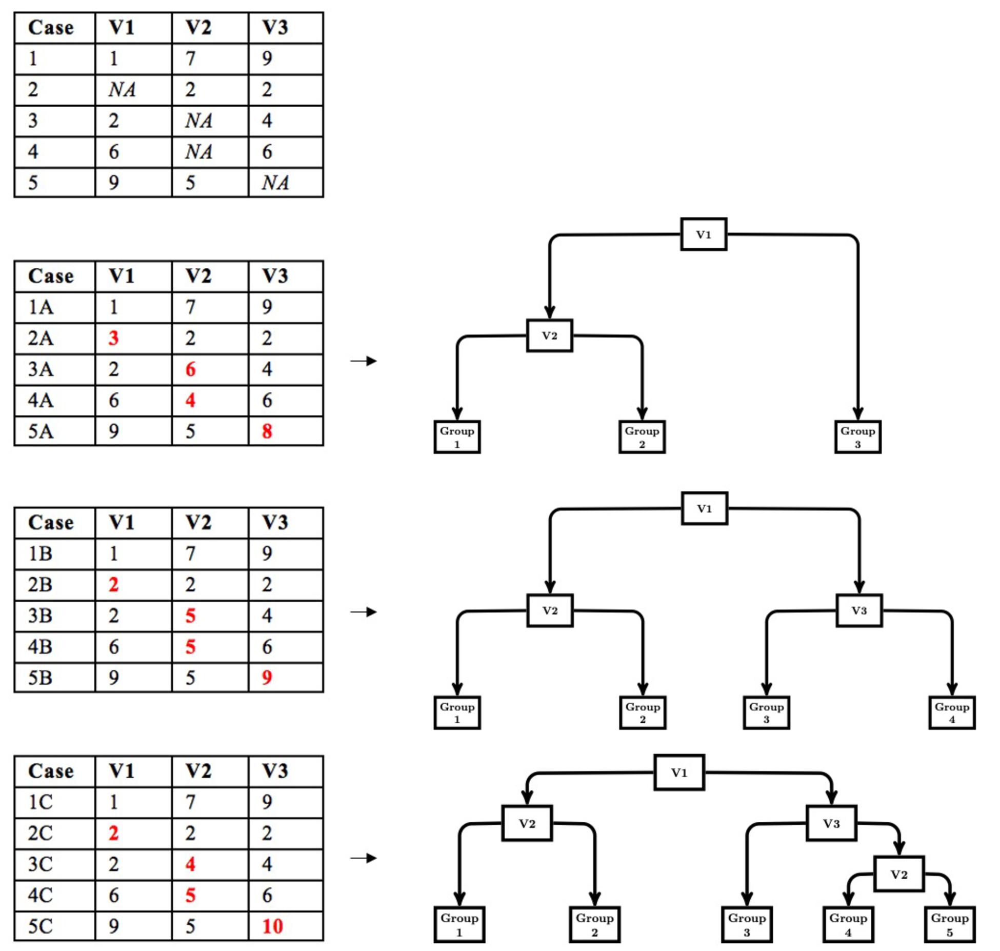
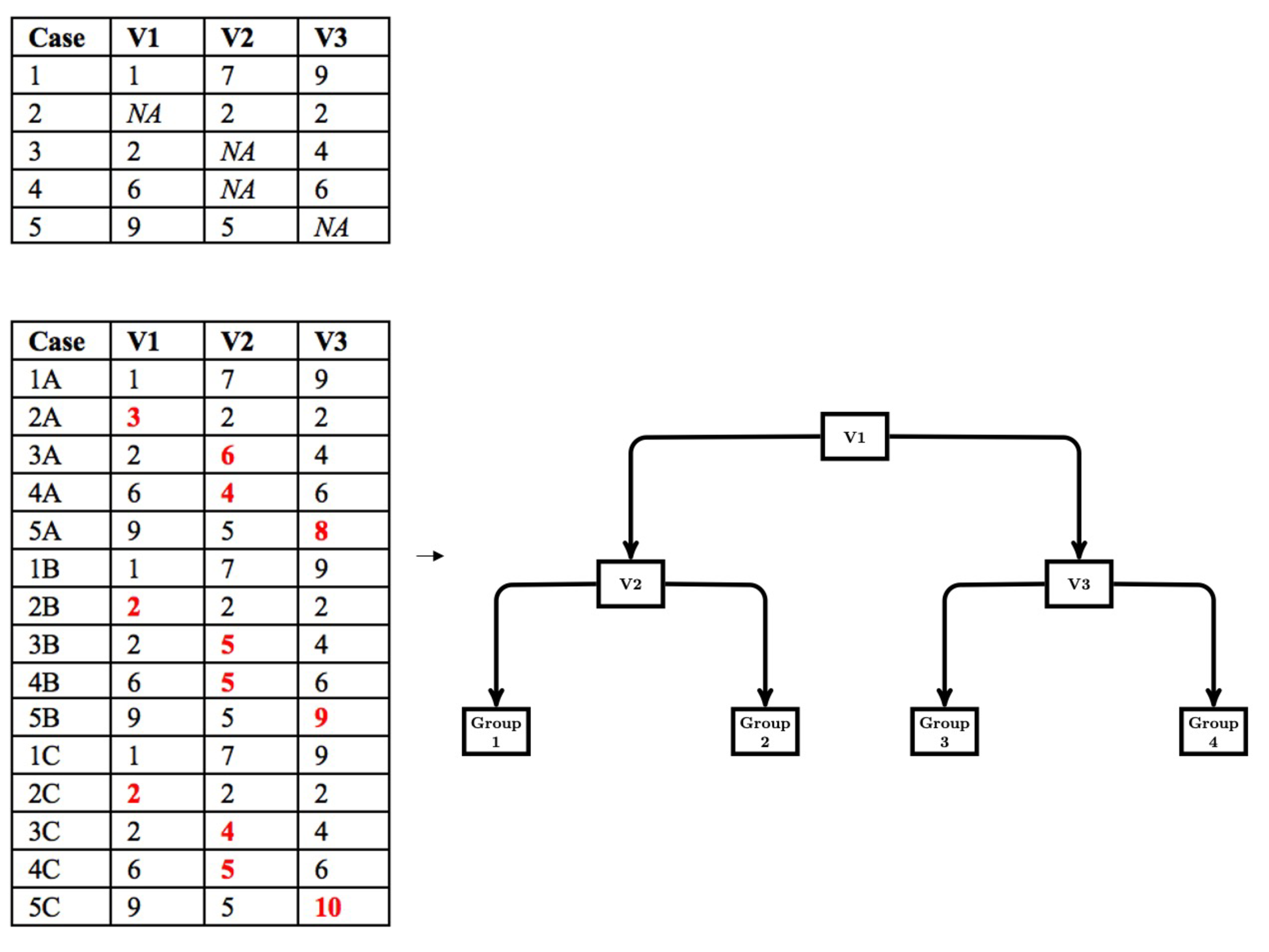
The modified multiple imputation approach for CART follows the first three steps of multiple imputation; however, the pooling step is different. First, data are imputed from a distribution specifically modeled for the missing data. Second, a CART is fit to the imputed data with the complexity parameter (cp) optimized using cost-complexity pruning through k-fold cross-validation. The cp controls the tree size for each imputed dataset. We use the cp to control tree size because the cp is used in rpart (Therneau & Atkinson, 2019), a common CART package available in R and the package we use in our simulation work. Other measures of tree size (e.g., depth) could be implemented based on availability. Third, the first two steps are repeated multiple times (e.g., 20). Figure 1 depicts a simple example of the first three steps. Fourth, the imputed datasets are stacked to create a single, large data set consisting of $m\cdot N$ rows, where $m$ is the number of imputed datasets and $N$ is the sample size for each imputed dataset. A CART is then fit to the stacked dataset with the cp set to the average of the optimized cp obtained when a CART was fit to each imputed dataset. Thus, in this pooling step, we pool the cp that controls tree growth and then use this value to fit a CART to the stacked data. This leads to a single DT that is indirectly optimized to the stacked multiply imputed dataset with a single set of decision rules that are easily interpreted (shown in Figure 2).
Fitting the final CART to the stacked multiply imputed dataset provides an optimal set of decision rules, but ignores the variability across imputed datasets. While imputation variability is an important component of the calculation of standard errors in the application of multiple imputation with a theoretically driven statistical model (e.g., multiple regression model), standard errors are not part of CART (and DTs more generally). The splitting values in CART are considered point estimates and CART does not provide information on the uncertainty of the point estimate.
Pooling the cp to control tree size is an important aspect of the modified multiple imputation approach. We note that the optimal cp cannot be determined through k-fold cross validation of the stacked multiply imputed data because the different folds of the data are too similar. For example, say we have a dataset with 10% MCAR missingness on ten variables. We conduct $m=20$ imputations and stack the multiply imputed data. Approximately 35% of the sample will have complete data leading to the same data appearing in the stacked data 20 times. Another 39% of the sample will be missing one value leading to 90% of their data appearing in the stacked data 20 times. The high degree of the same data appearing in the dataset is problematic for k-fold cross-validation because the data from k$-1$ folds that are used to train the algorithm are too similar to the data in the k$^{th}$ fold that is used to test the model. Thus, using k-fold cross validation with the stacked multiply imputed data leads to an overgrown (overfit) CART. Determining tree size based on pooling the cp leads to more appropriately sized DTs.
Next, we conduct a Monte Carlo simulation study to examine the performance of the modified multiple imputation approach outlined above and compare its performance to the missing data methods currently implemented with DTs in terms of its predictive performance, variable selection, variable importance, and tree size.
A Monte Carlo simulation study was conducted to compare how well the different missing data approaches performed with CARTs. Data were generated from a population tree structure, missing values were generated following different missing data protocols, CARTs were fit to these datasets using each missing data handling approach, and we examined various indices of the resulting prediction model. This process was repeated 1,000 times for every condition. Baseline measures were taken from complete datasets (i.e., containing no missing values) and used for comparison. We examined the performance of each missing data approach with respect to prediction accuracy, variable selection, and variable importance. All programming scripts are contained on the third author’s website.
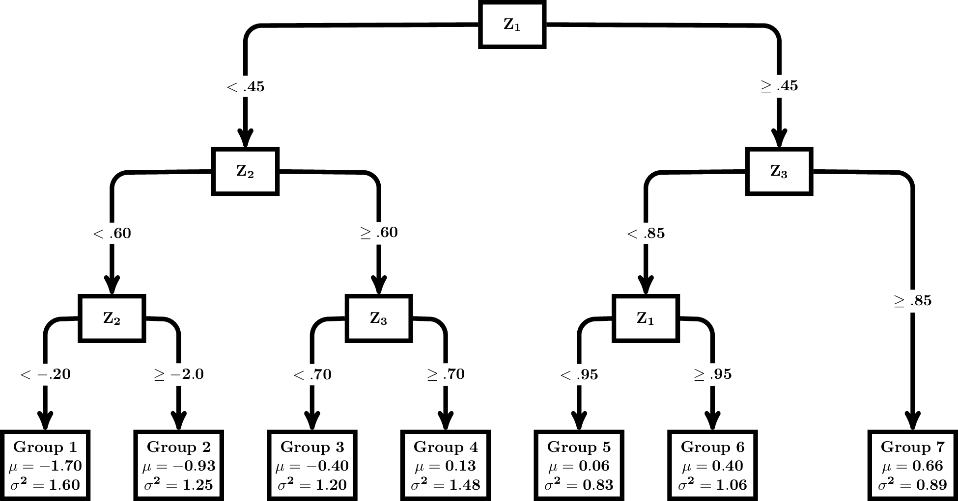
Data were generated using R (R Core Team, 2020). All predictor variables were independently drawn from a standard normal distribution (i.e., $\mu $=0, $\sigma $=1). Depending on the condition, one ($x_{1}$) or four ($x_{1}$, $x_{2}$, $x_{3}$, $x_{4}$) variables were created. Three predictor variables, $z_{1}$, $z_{2}$, and $z_{3}$, were then generated to either correlate .4 or .6 with the $x$ variables, and $z_{1}$, $z_{2}$, and $z_{3}$, were subsequently used to generate the outcome using a series of decision rules from a population DT. The population tree structure included six splits and seven terminal nodes. The outcome variable, $y$, was generated from the population tree shown in Figure 3 with values generated from a normal distribution with the mean and variance reported in each terminal node. Of note, the first split in the population tree was on $z_{1}$. Additionally, six distractor predictor variables, $z_{4}$ through $z_{9}$ were generated from a standard normal distribution and correlated .15 with $z_{1}$, $z_{2}$, and $z_{3}$. Each simulated dataset included 10 or 13 predictor variables (i.e., three used in the population DT, one or four used for missing data generation, and six distractors), and the outcome variable.
Manipulated features included sample size and characteristics of missing values. The sample sizes considered were $N$ = 200, $N$= 500, or $N$= 1,000 to cover a range of sample sizes common in the social and behavioral sciences. Missing values were imposed across all predictors, but they were not imposed on the outcome variable. The nature of the missing values only varied for $z_{1}$, which was the first splitting variable in the population tree structure. The missing data mechanism was varied, the percentage of missing data, the number of variables that the likelihood of a missing value was dependent on, and the degree of association between the likelihood of missingness and the other variable(s) in the dataset. Missing data generation on all other predictors (all predictor variables excluding $z_{1}$) were MCAR with a 2.5% probability of being recorded as missing.
The method for imposing missing values on $z_{1}$ closely followed methods from Mazza, Enders, and Ruehlman (2015). Missing values were designed to either be missing at random (MAR) or missing completely at random (MCAR). In the MAR condition, missing values on $z_{1}$ were generated to relate to one ($x_{1}$) or four variables ($x_{1}$, $x_{2}$, $x_{3}$, and $x_{4}$). The association between the likelihood of missingness and the other variable(s) in the dataset was specified using a logistic regression model (Agresti, 2012; Johnson & Albert, 1999; Mazza et al., 2015), with slope and intercept parameters chosen to produce the desired level of association between the underlying missingness probability and the complete variable(s) as well as the overall percentage of missing values. Slopes were selected such that the strength of association between the underlying missingness probability and the complete variable(s) was either $R^{2}$ = .2 for a moderate association or $R^{2}$ = .4 for a strong association. Intercepts were selected so that the percentage of missing values on $z_{1}$ was either 15% or 30%, which are rates commonly found in psychological and educational research (Enders, 2003). The MCAR condition had fewer manipulated features than the MAR conditions because missingness was unrelated to any other variables in the dataset. Since MCAR occurs when the likelihood of missingness occurs at random, the slope for the logistic regression model was 0 and intercepts were chosen such that the percentage of missing values was either 15% or 30% on $z_{1}$.
Listwise deletion, delete if selected, majority rule, surrogate splits, single imputation, multiple imputation with prediction averaging, and the proposed multiple imputation approach were used to handle the missing data. Listwise deletion was employed by deleting cases with missing values prior to analyses. Delete if selected was applied using the control settings (i.e., usesurrogate=0) from the rpart package (Therneau & Atkinson, 2019) in R (R Core Team, 2020). Majority rule was also employed using the control function by specifying that no surrogates would be used in the analyses (i.e., maxsurrogate=0). By setting the max number of surrogates in the analysis to zero (maxsurrogate=0), the algorithm was forced to assign cases with missing values based on majority rule. Delete if selected control setting specifies that the surrogate split method would not be used to treat missing data (usesurrogate=0). The surrogate split approach used the default method (i.e., usesurrogate=2) to place observations with missing values. If no surrogates were found, then majority rule was enacted.
For single and multiple imputation, data were imputed using the Multivariate Imputation by Chained Equations (mice) package (van Buuren & Groothuis-Oudshoorn, 2011) in R (R Core Team, 2020). The elementary imputation method was specified using program defaults, which used predictive mean matching. In the single imputation approach, missing values were imputed once to create a single dataset (i.e., $m$ = 1), which was then analyzed. In the multiple imputation approaches, missing values were imputed 20 times (i.e., $m$ = 20). According to van Buuren and Groothuis-Oudshoorn (2011), mice assumes that the multivariate distribution of an incomplete variable is completely specified by a vector of unknown parameters, $\theta $. Sampling iteratively, the algorithm models the conditional distributions of the incomplete variable given the other variables to obtain a posterior distribution of $\theta $. Using Gibbs sampling, the algorithm selects and fills in plausible values for the missing values on the incomplete variables. Outcome distributions are assumed for each variable instead of the whole dataset. The chained equations within mice refer to concatenating univariate procedures to fill in missing data (van Buuren & Groothuis-Oudshoorn, 2011).
DTs recursively partitions data until one of the stopping criteria is reached for each node. Optimal tree sizes were determined using a two-step procedure for listwise deletion, delete if selected, majority rule, surrogate splits, and single imputation. First, all stopping criteria were set to small values to generate an overgrown tree. For all splits in this overgrown tree, 10-fold cross-validation was used to determine the relative cross-validation prediction error associated with the split. The tree was then pruned by specifying the cp associated with the smallest estimate of cross-validated prediction error from the 10-fold cross-validation. In multiple imputation, each imputed dataset was analyzed separately and each tree was overgrown. The cp associated with the optimal tree size determined through 10-fold cross-validation was retained. In multiple imputation with prediction averaging, the predicted values from each pruned tree were averaged. In the modified multiple imputation approach, the multiply imputed data were stacked and analyzed with the cp set to the average value of the cp obtained when the CART was fit to each imputed dataset separately.
There are several viable approaches to choosing tuning parameters in machine learning. This study used the minimum cross-validated prediction error to determine the best model that would optimize prediction accuracy. However, it is important to note that methods like the “one standard error” rule (Breiman et al., 1984) are often used in practice. The “one standard error rule” uses the most parsimonious model whose error is no more than one standard error above the error of the best model (Hastie, Tibshirani, & Friedman, 2009).
Four evaluation metrics were examined to assess and compare the performance of the missing data approaches. The metrics were the averaged mean square error (MSE) in a test dataset, the proportion of replicates where the first splitting variable was $z_{1}$, variable importance metrics, and the median number of splits.
The final DT from each missing data approach was used to generate predicted values in the test dataset with $N$ = 10,000 drawn from the same population. The test dataset contained no missing values, and was not used to estimate any of the models. The predicted values in the test dataset were calculated and used to determine the MSE - a measure of prediction accuracy. Lower MSE values indicated stronger prediction accuracy, whereas higher MSE values indicated weaker prediction accuracy. The performance of missing data approaches was compared to each other and with the CART estimated using the complete data.
The second evaluation metric was proportion of replicates where $z_{1}$ was the first variable selected to split the data. Recall that variable $z_{1}$ was the first spitting variable in the population tree. Thus, the proportion of times $z_{1}$ (i.e., the target variable) was correctly selected for the first split indicates the CART properly selected the primary splitting variable. The third evaluation metric was variable importance. Variable importance assesses the degree to which each variable contributes to the prediction of the outcome. Variable importance is calculated for every predictor by summing together the decrease in error for every split using the variable as the splitting variable. We assessed and compared variable importance values for $z_{1}$, $z_{2}$, and $z_{3}$ across each missing data approach, and compared variable importance to the values obtained when analyzing the complete data.
The median number of splits was the last evaluation metric. Seven decision trees were fit (i.e., complete data and the six missing data approaches) for each replication within a condition. The median number of splits across all replications within a condition was recorded for each approach. This was compared across missing data approaches and compared to the number of splits in the population DT as an indication of proper tree size.
Overall, the proposed multiple imputation approach and surrogate splits performed well across all outcome measures. The proposed multiple imputation approach (closely followed by single imputation) performed best when data were MAR with multiple variables strongly predicting missing values and strong associations among predictors. Surrogate splits performed well when data were MCAR or MAR with a single variable predicting missing values and weak associations among predictors. Other approaches stood out on specific outcomes. For example, multiple imputation with prediction averaging had the greatest prediction accuracy. Listwise deletion correctly selected $z_{1}$ for the first split more often than all other approaches. However, these methods only performed well on specific outcomes and not across all outcome measures. The following sections summarize and compare the approaches for each outcome.
MSE values for each missing data approach are shown in Figure 4 for four representative conditions. The conditions were selected to represent (1) a mild MCAR condition (i.e., 15% missingness and predictors correlated .16), (2) a mild MAR condition (i.e., 15% missingness, weak association among predictors and missing values ($R^{2}$ = .2), a single predictor of missingness, predictors correlated .16), (3) a moderate MAR condition (i.e., 30% missingness, greater association among predictors and missing values ($R^{2}$ = .4), a single predictor of missingness, predictors correlated .36), and (4) a severe MAR condition (i.e., 30% missingness, greater association among predictors and missing values ($R^{2}$ = .4), multiple predictors of missingness, predictors correlated .36).
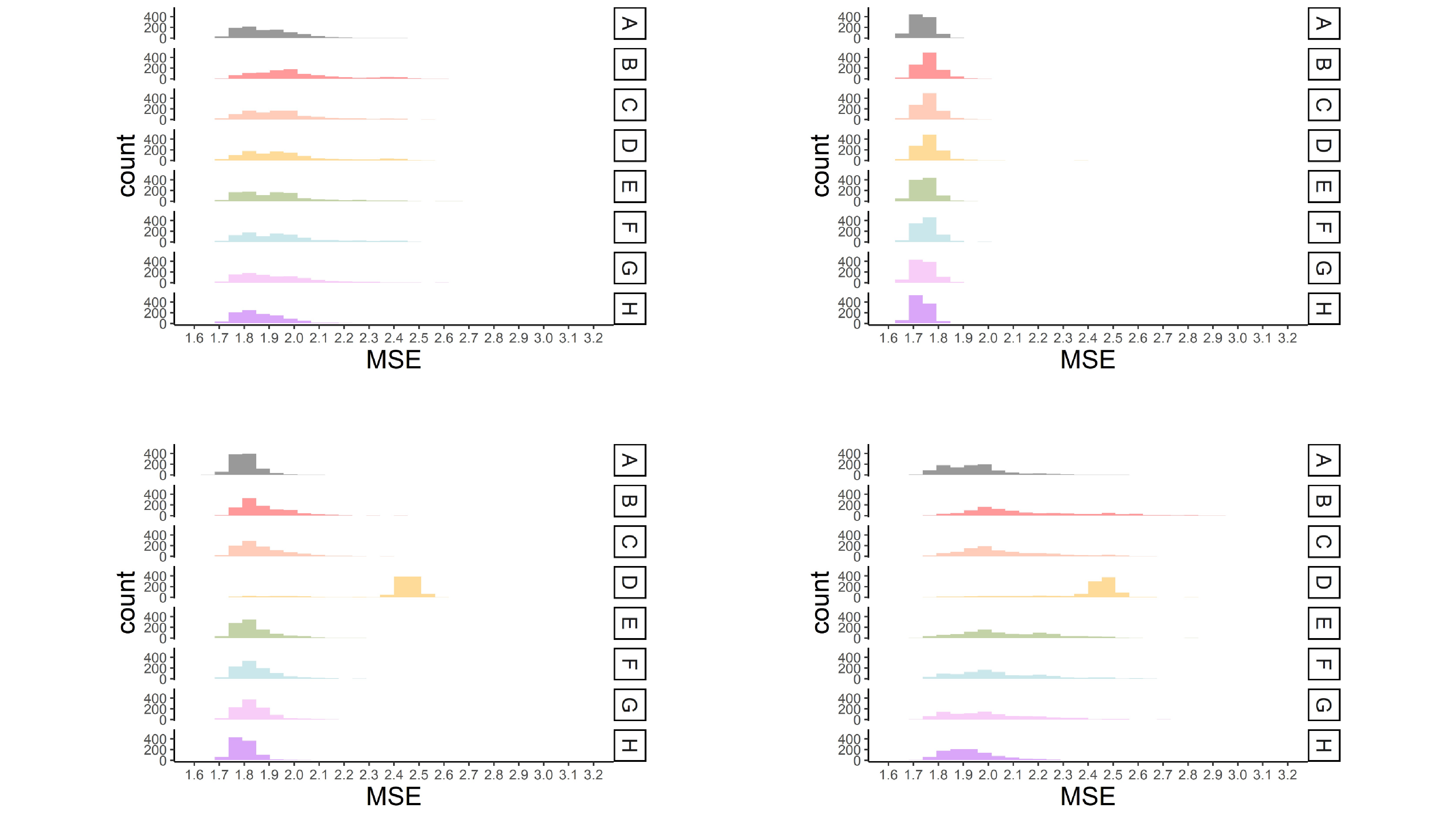
Overall, a higher percentage of missing data led to higher MSE across all approaches for handling missing data. This effect was greater in the smaller sample size conditions. Multiple imputation with prediction averaging produced the least amount of bias, which was likely because this approach is an ensemble-type approach like bagging (Breiman, 1996). The average MSE for this approach most closely resembled the results when the CART was fit to the complete data (see Figure 4). The proposed multiple imputation approach and surrogate splits produced more bias than the multiple imputation approach with prediction averaging. Differences between the proposed approach and surrogate splits were minimal (i.e., average MSE typically only differed by .01) and became less apparent in the larger sample size conditions. The proposed multiple imputation approach produced less bias than surrogate splits when there were multiple predictors of missingness, stronger associations between predictors and missingness, and a higher percentage of missing data (fourth panel in Figure 4). This approach generally handled small sample sizes ($N$ = 200) better than surrogate splits across all MAR conditions.
Surrogate splits often produced the same amount of bias as the proposed multiple imputation approach when data were MCAR and in the MAR conditions with a single predictor of missingness and weaker associations between variables and missingness (first and second panel in Figure 4). Overall surrogate splits produced less bias than the proposed approach across these mild missing data conditions (see Table S1 in supplemental materials). Single imputation closely followed the proposed multiple imputation approach and surrogate splits but had slightly greater average MSE values. Also, single imputation performed fairly well in the conditions where missingness was related to multiple predictors. Delete if selected and listwise deletion produced slightly greater bias across all the conditions and majority rule produced the greatest amount of bias across all conditions.
The proportion of times that $z_{1}$ was chosen for the first split was recorded. Figure 5 illustrates the performances of each approach in four example conditions that range from mild to severe missing data conditions in this simulation. Across all approaches, higher rates of missing values led to fewer instances that $z_{1}$ was chosen for the first split. Greater effects were found in small sample sizes. Conditions represented in Figure 5 have a consistent sample size and rate of missing to simplify comparisons across missing data patterns and associations.
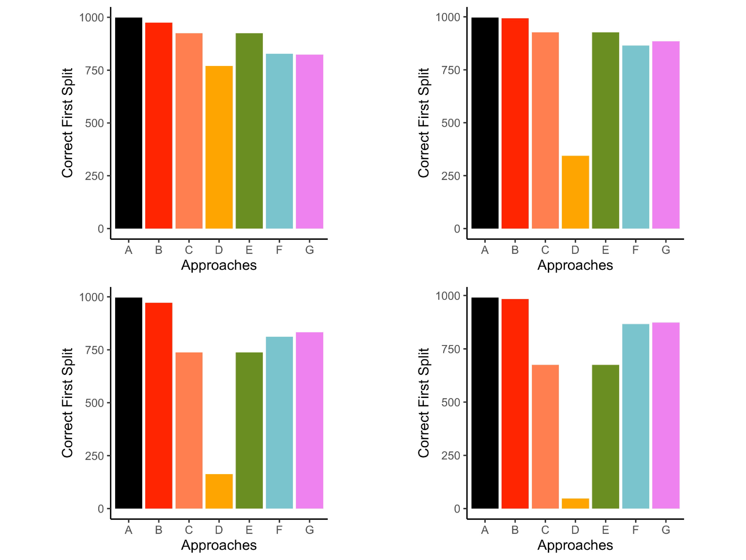
Listwise deletion correctly selected first split more frequently than the other approaches and most closely resembled the complete data conditions (see Figure 5). The performance of the other approaches depended on the missing data pattern, strength of association among predictors and missing values, and the percentage of missing data. When data were MCAR, surrogate splits and delete if selected correctly chose $z_{1}$ for the first split more often than the remaining approaches (first panel in Figure 5).
Performance across the MAR conditions depended on the strength of association among predictors and percent missingness. When there were weak associations between predictors and missing values (i.e., association between $z_{1}$, $z_{2}$, $z_{3}$ and $x$ variables used to generate missing values) and only 15% missing data, the proposed multiple imputation approach selected $z_1$ more often than all other approaches with the exception of listwise deletion. However, delete if selected and surrogate splits outperformed the proposed multiple imputation approach in the same conditions with 30% missing data (second panel in Figure 5). This pattern of results can be found in supplemental materials (see Table S2 in supplemental materials). When there were strong associations between the predictors and variables used to generate missing values, the proposed multiple imputation approach correctly selected $z_{1}$ more frequently than the remaining approaches, such as single imputation, delete if selected, surrogate splits, and majority rule (fourth panel in Figure 5).
Averaging the proportion of correct first variable splits across all conditions leads to the following set of results. In the complete data conditions, $z_{1}$ was selected for the first split 98% of the time. Listwise deletion correctly identified the first split 94% of the time, which was more often than the other approaches (Table 1). The proposed multiple imputation approach correctly selected $z_{1}$ for the first variable split 88% of the time, whereas single imputation averaged 87%. Delete if selected slightly outperformed surrogate splits, but both approaches were nearly identical in correctly selecting the variable for first split 85% of the time. Majority rule selected the correct variable for the first split 56% of the time. Multiple imputation with prediction averaging did not produce a single tree structure, so this outcome was not evaluated for this approach.
|
|
|
|
|
|
|
||||||||||||||
| .980 | .941 | .848 | .562 | .854 | .873 | .882 | ||||||||||||||
Variable importance values ranged from 0 to 1 for $z_{1}$, $z_{2}$, and $z_{3}$. Recall that $z_{1}$ was the target variable that contained missing values, was the first variable split, which is often associated with the greatest variable importance values. In conditions where the data were MCAR, listwise deletion most closely mimicked the variable importance values from the complete data conditions (see the left panel of Figure 6). Surrogate splits performed well, but tended to overestimated the importance of $z_{1}$ and $z_{2}$, and underestimated the importance of $z_{3}$, especially with larger sample sizes. The single and proposed multiple imputation approaches performed moderately well and produced nearly identical results. Both approaches underestimated the importance of $z_{1}$ and slightly overestimated the importance of the other predictors. The delete if selected and majority rule approaches mimicked the pattern for surrogate splits, but had greater discrepancy in overestimating the importance of $z_{1}$. Majority rule consistently performed poorly with respect to this outcome compared to the other missing data handling approaches.
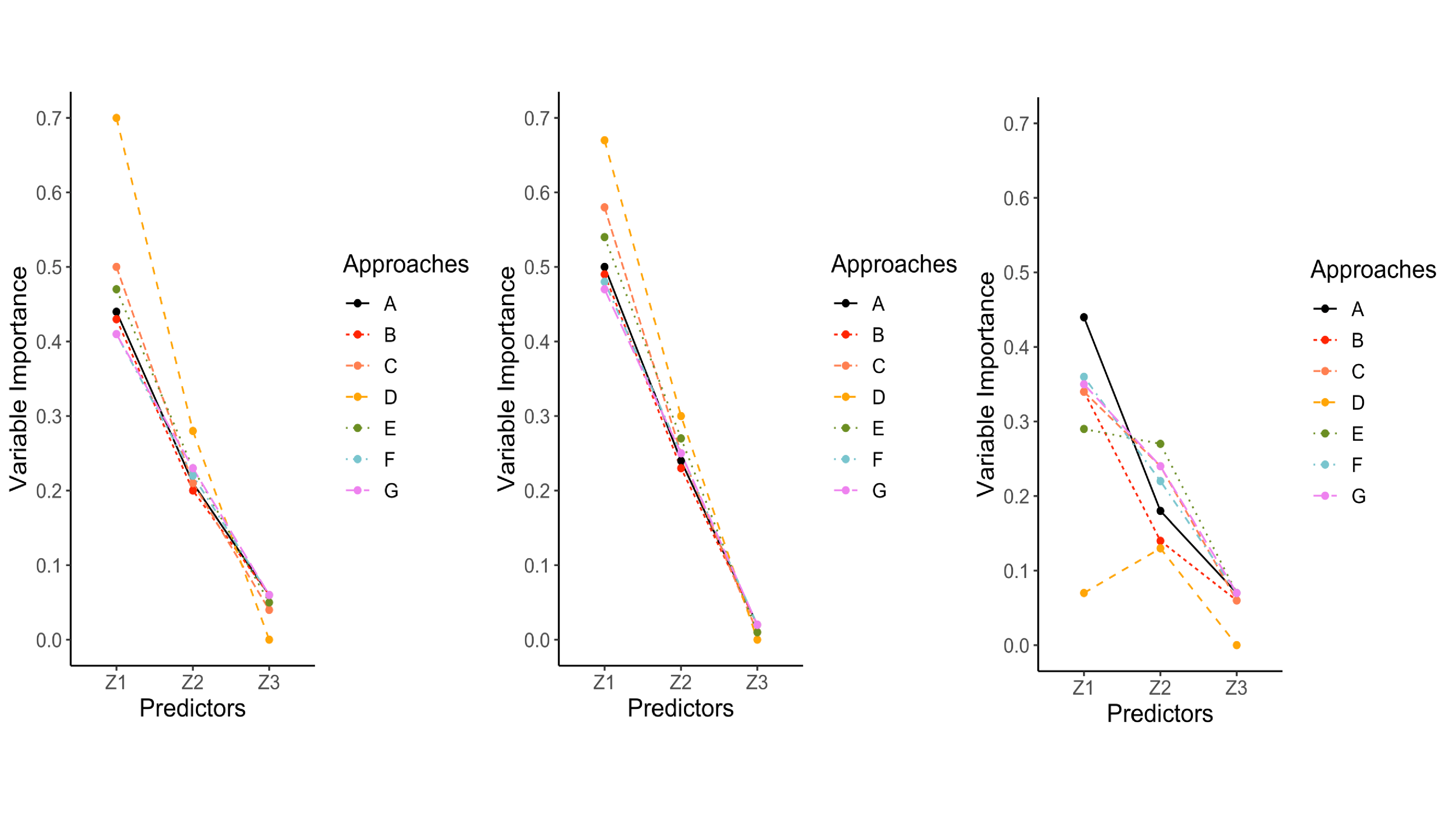
The results for variable importance revealed a distinction between the MAR conditions. MAR conditions with a single variable predicting missing values and weak associations among variables had similar results when compared to MCAR conditions. However, in the more severe MAR conditions (i.e., multiple variables predicting missing values, stronger association among predictors, high percentage of missing data), single imputation started to outperform the other approaches. Single imputation still underestimated the importance of $z_{1}$ and overestimated the other variables, but this approach had small discrepancies when compared to the complete data conditions. The proposed multiple imputation approach and delete if selected closely followed single imputation. Listwise deletion followed the same trajectory as the complete data but underestimated the importance of all predictors with larger discrepancies. Surrogate splits performed poorly in the most severe MAR conditions because it largely underestimated the importance of $z_{1}$ and overestimated the importance of $z_{2}$ (third panel in Figure 6). Majority rule consistently had the greatest discrepancies (shown in Figure 6).
The median number of splits for each DT was recorded. The population tree contained six splits. The median number of splits across each approach ranged from zero to four indicating that each DT tended to underfit the data. There were little differences among most approaches across conditions. Complete data, listwise deletion, delete if selected, surrogate splits, and single imputation all had a median of two splits. The proposed multiple imputation approach often averaged one more split than the other approaches in the large sample size conditions ($N$ = 1,000), but the overall differences were minimal. Majority rule approach averaged two splits in most conditions, but failed to find any variable to predict the outcome (i.e., resulting in zero splits) when there was a high percentage of missing values that were MAR. Multiple imputation with prediction averaging did not produce a single DT structure, so the median number of splits was not recorded.
Data were drawn from the Head Start Family and Child Experiences Survey 1997-2001 (FACES1997) study. The goals of FACES1997 were to (1) examine whether Head Start enhances children’s development and school readiness, (2) evaluate whether Head Start strengthens families as the primary nurturers of their children, (3) determine whether Head Start provides children with high quality educational, health, and nutritional services, and (4) determine how Head Start classroom quality is related to children’s outcomes. FACES1997 is a longitudinal study of 1,968 children enrolled in a Head Start program in 1997 with data collected on the cognitive, social, emotional, and physical development of Head Start children, characteristics and opinions of Head Start teachers, and characteristics and evaluations of Head Start classrooms (https://www.childandfamilydataarchive.org/cfda/archives/cfda/studies/4134).
The analytic sample contained $N$ = 785 children who were in first grade during the 1999-2000 school year and completed cognitive testing in the spring of 2000. Of these 785 children, 370 (47%) were female. The sample was diverse with respect to race/ethnicity. Twenty-nine percent of this subsample identified as white (non-Hispanic), 39% black (non-Hispanic), 1% Asian or Pacific Islander, and 2% Native American Indian or Alaskan. Thirty-two percent of the sample identified as Hispanic. Seventy-one percent were living below the poverty line determined by an income-to-needs ratio less than 1.0. Seventy-seven percent of families reported that at least one parent obtained a 12th grade education (e.g., graduated from high school, received a GED).
These data were split into training and testing samples using a 60-40 split. Given the focus of the paper, the testing sample had complete data to make model evaluation clean, and the training data contained missing values. The training data were analyzed to develop statistical models using different missing data handling methods. DTs were overgrown and then pruned using cost-complexity pruning and $k$-fold cross-validation following the approach in our simulation work. Once an optimal model was determined for the training data, the model was used to generate predicted values in the testing dataset and the MSE was calculated.
The outcome variable was the Peabody Picture Vocabulary Test (PPVT; Dunn & Dunn, 1981) standard score, which was measured in the spring of 2000. Predictor variables included a series of assessments collected during Head Start in the fall of 1997. These assessments were academic (e.g., Woodcock-Johnson Letter-Word Identification) or social (e.g., Social Skills Rating Scale) in nature.
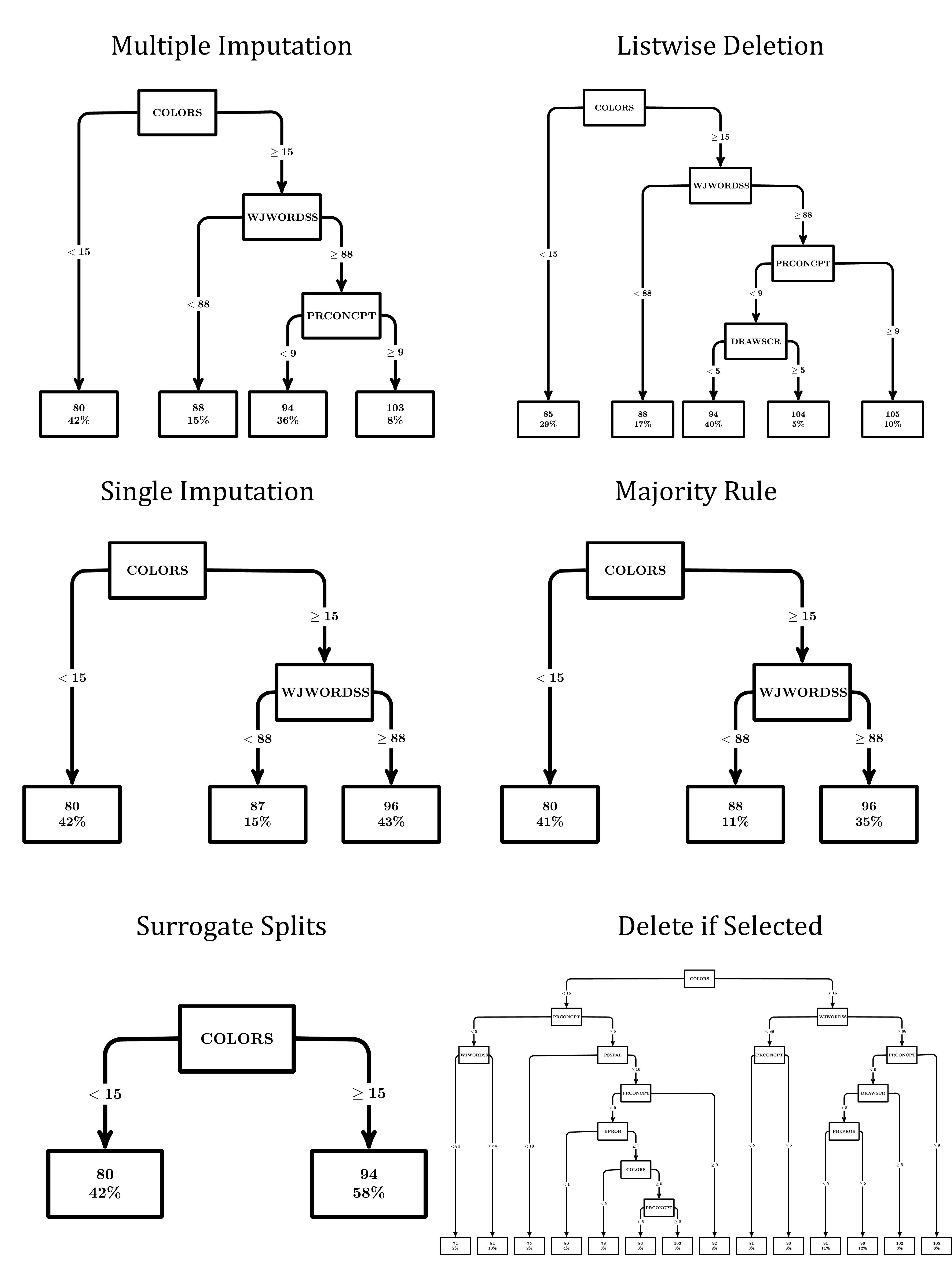
The DTs from each missing data handling method are shown in Figure 7. Each terminal node contains the predicted value of the PPVT and the percent of the sample in the node. The predictor variable used to split the data is labeled within each tree node and split values are presented within the tree branches. Overall, DTs varied across methods. Note that multiple imputation with prediction averaging did not produce a consistent tree structure, so it is not included in Figure 7. For the remaining approaches, the number of splits across DTs ranged from 1 to 13. However, many of the resulting trees shared splitting variables and values. In all remaining missing data approaches, the first splitting value was a score of 15 on identifying colors by name (COLORS). The tree produced from the surrogate split approach contained no subsequent splits. For all other approaches, the node for participants with identifying colors by name greater than or equal to 15 was split based on a value of 88 on the Woodcock-Johnson Letter-Word Identification (WJWORDSS; Woodcock & Johnson, 1989). Notably, majority rule and single imputation had identical tree structures and did not contain any further splits. Delete if selected, listwise deletion, and the modified multiple imputation approach shared another common split value of nine on print concepts (PRCONCEPT). The DT using the modified multiple imputation approach did not contain any additional splits, whereas the listwise deletion approach contained one additional split at the value of five on McCarthy Drawing Test score (DRAWSCR; McCarthy, 1972). Lastly, the delete if selected approach contained several additional splits beyond those described above (shown in Figure 7).
Variable importance measures for the predictors for each DT are shown in Table 2. There was agreement across many of the missing data approaches. All missing data approaches that produced variable importance measures emphasized COLORS as an important predictor. On the other hand, a few variables were highlighted among most, but not all, missing data approaches. For example, all the approaches that were evaluated, except surrogate splits, indicated that WJWORDSS was an important variable. Nearly all approaches highlighted print concepts, The McCarthy Drawing Test score, book knowledge (BOOKKNLG), social awareness (SAWARE), and the Child Behavior Problems Index (PBEPROB; Peterson & Zill, 1986) as important variables in all DTs, with majority rule as the exception. The last three predictors were only highlighted by a few approaches. Social skills (SSRS; Gresham & Elliott, 1990) was deemed important with listwise deletion, delete if selected, and surrogate split approaches, whereas social skills/positive approach to learning (PSSPAL) was considered important using listwise deletion, delete if selected, and single imputation. Behavior problems total score (BPROB) was uniquely selected as an important predictor by the delete if selected approach. In summary, all approaches agreed on the variable of greatest importance (i.e., COLORS), and six out of the ten remaining predictors were highlighted in DTs using different missing data approaches.
| Predictors |
|
|
|
|
|
|
||||||||||||
| COLORS | 0.34 | 0.37 | 0.86 | 0.55 | 0.46 | 0.44 | ||||||||||||
| WJWORDSS | 0.21 | 0.07 | 0.14 | - | 0.14 | 0.12 | ||||||||||||
| PRCONCPT | 0.21 | 0.22 | - | 0.13 | 0.12 | 0.17 | ||||||||||||
| DRAWSCR | 0.09 | 0.04 | - | 0.04 | 0.04 | 0.03 | ||||||||||||
| BOOKKNLG | 0.08 | 0.11 | - | 0.11 | 0.10 | 0.11 | ||||||||||||
| SAWARE | 0.03 | 0.10 | - | 0.14 | 0.13 | 0.12 | ||||||||||||
| PBEPROB | 0.02 | 0.01 | - | - | 0.01 | $<$0.01 | ||||||||||||
| SSRS | 0.02 | 0.03 | - | 0.03 | - | - | ||||||||||||
| PSSPAL | 0.01 | 0.02 | - | - | $<$0.01 | - | ||||||||||||
| BPROB | - | 0.02 | - | - | - | - | ||||||||||||
| BEARCNT | - | - | - | - | - | - | ||||||||||||
Predictions from each DT were generated for the test data. Test data contained no missing values and consisted of 314 participants. To evaluate prediction accuracy, the MSE (i.e., average squared difference of estimated scores from DTs and actual scores on test data) was calculated for each missing data approach (see Table 3). Overall, listwise deletion produced the best prediction of PPVT in the test data. The proposed multiple imputation approach had the second-best performance. Majority rule, single imputation, and multiple imputation with prediction averaging performed similarly to the proposed multiple imputation approach with only minor increases in MSE. Delete if selected performed poorly, and surrogate splits had the poorest performance.
| Measures |
|
|
|
|
|
|
|
|||||||||||||
| MSE | 134.60 | 149.85 | 145.16 | 156.24 | 146.07 | 144.00 | 146.17 | |||||||||||||
| $R^2$ | 0.37 | 0.35 | 0.36 | 0.25 | 0.36 | 0.37 | 0.33 | |||||||||||||
Note. SI: Single Imputation.
We also calculated an $R^{2}$ value to measure predictive quality of each missing data approach (shown in Table 3). Specifically, $R^{2}$ was calculated as the squared correlation between the predicted and observed outcome values using the test data. It represents the percent of variance in test data PPVT scores accounted for by the prediction model using each missing data approach. Thirty-seven percent of the variance in PPVT scores was accounted for by the predicted values produced by the listwise deletion approach. Similarly, 37% of the variance in PPVT scores was accounted for by predicted scores from the modified multiple imputation approach. Single imputation and majority rule approach led to $R^{2}$ values of 36% and delete if selected led to an $R^{2}$ of 35%. Multiple imputation with prediction averaging had an $R^{2}$ of 33% and the DT using surrogate splits had an $R^{2}$ of 25%. In summary, listwise deletion and the modified multiple imputation approach led to DTs that performed best in the test dataset.
A modified multiple imputation approach was proposed for handling missing data in DTs. The proposed approach involves four steps: (1) Impute missing values, (2) Fit a DT to the imputed dataset, prune the DT using k-fold cross validation, and retain the associated cp value, (3) Repeat steps 1 and 2 multiple times, and (4) stack all imputed datasets into a single data frame, fit a DT to the stacked dataset, and using the averaged cp value from when the DTs were fit to each imputed dataset. A simulation was conducted to compare the proposed approach to listwise deletion, delete if selected, majority rule, surrogate splits, single imputation, and multiple imputation with prediction averaging under multiple MAR and MCAR conditions.
Overall, all missing data approaches produced DTs with better performance in conditions with larger sample sizes and lower rates of missing values. Across the outcome measures, the proposed multiple imputation method performed better than the other approaches when data were MAR with a strong association between multiple predictors and missing values. Additionally, the proposed multiple imputation approach handled small sample sizes ($N$ = 200) better than the other approaches across the MAR conditions. On the other hand, surrogate splits performed the best when data were MCAR and when data were MAR with a single predictor that had a weak association with missing values. It appears the weak associations in these MAR conditions led to conditions that were close to MCAR.
In addition to the simulation work, empirical data from FACES 1997-2001 were analyzed to compare the seven approaches for handling missing data. A series of assessments were taken on a total of $N$ = 785 children. We found that listwise deletion and multiple imputation had the highest prediction accuracy as measured by MSE and $R^{2}$. Majority rule, single imputation, and delete if selected had relatively high prediction accuracy. Surprisingly, multiple imputation with prediction averaging had lower prediction accuracy and surrogate splits had the worst prediction accuracy.
The results of our simulation research leads to the following set of recommendations. The proposed multiple imputation approach is recommended in situations where data are MAR, especially when dealing with small sample sizes. Surrogate splits are recommended when data are MCAR or mildly MAR (i.e., data are MAR with weak associations and a fairly large sample sizes, $N \ge $ 500). If a researcher is only interested in prediction accuracy and has no interest in interpreting the DT, multiple imputation with prediction averaging is recommended for either MAR and MCAR data. However, in these situations, an ensemble method, such as random forests (Breiman, 2001) or boosting (Breiman, 1998; Friedman, 2002), may be preferred. Single imputation is a simple approach, but is not recommended over the proposed multiple imputation approach because it often underperformed by comparison.
Listwise deletion, delete if selected, and majority rule are not generally recommended. Both listwise deletion and delete if selected could be recommended when data are MCAR and there is a small percentage of missing data. Deletion approaches may be a relatively simple and convenient method for handling missing data in such situations, but these methods proved inferior in most conditions. Majority rule generally had the poorest performance across all conditions and is not recommended.
A limitation of this study is that missing data were handled with a single type of imputation. A variety of imputation methods have been developed in statistical frameworks, which are typically built upon linear or logistic regression models. However, imputation models have also been built upon partitioning algorithms, such as DTs and random forests (Tang & Ishwaran, 2017), and these imputation approaches were not considered.
A second limitation is that we only considered one pooling approach in the proposed multiple imputation approach. That is, when analyzing the stacked multiply imputed dataset, the cp was set to the average value obtained from analyzing each imputed dataset. Another metric may be more appropriate instead of the average. For example, the minimum value of the cp or the 5th percentile would lead to larger DTs and may be more appropriate because the resulting DTs were smaller than the population DT. More research is needed to determine the optimal approach to determining the size of the DT with the stacked multiply imputed data.
Another consideration is that this study evaluated how well missing data approaches performed when the predictors contain missing values and the outcome variable does not. The nature of the missing values was manipulated only on the first splitting variable, $z_{1}$. However, in practice, missing values may appear across both the predictors and outcome variable. Future studies should consider how to treat the case where values on the outcome variable are missing.
The proposed modified multiple imputation approach for handling missing data in DTs was found to outperform surrogate splits, the default approach in several DT packages, for handling MAR data, particularly in small samples. To our knowledge, multiple imputation has only been implemented in DTs by averaging predicted values from different tree structures fit to each imputed dataset (Feelders, 1999; Twala, 2009). Our proposed modified multiple imputation approach leads to a single DT so that a single set of splitting variables can be interpreted.
Machine learning techniques are becoming more widely accepted in the social and behavioral sciences where missing data are a common problem. Additional research is needed to more fully examine how different machine learning algorithms, including different DT algorithms, such as conditional inference trees (Hothorn, Hornik, & Zeileis, 2006) and evolutionary trees (De Jong, 2006; Eiben, 2003; Fogel, Bäck, & Michalewicz, 2000), perform under a variety of missing data conditions and whether novel missing data approaches can improve upon the default strategies. We look forward to this research.
Agresti, A. (2012). Categorical data analysis (3rd ed.). Wiley.
Allison, P. (2002). Missing data. SAGE Publications, Inc.
Baraldi, A. N., & Enders, C. K. (2010). An introduction to modern missing data analyses. Journal of School Psychology, 48(1), 5-37. doi: https://doi.org/10.1016/j.jsp.2009.10.001
Batista, G. E. A. P. A., & Monard, M. C. (2003). An analysis of four missing data treatment methods for supervised learning. Applied Artificial Intelligence, 17(5-6), 519-533. doi: https://doi.org/10.1080/713827181
Beaulac, C., & Rosenthal, J. S. (2020). Best: A decision tree algorithm that handles missing values. Computational Statistics, 35(3), 1001–1026. doi: https://doi.org/10.1007/s00180-020-00987-z
Breiman, L. (1996). Bagging predictors. Machine Learning, 24(2), 123-140. doi: https://doi.org/10.1007/bf00058655
Breiman, L. (1998). Arcing classifiers. The Annals of Statistics, 26(3), 801–824.
Breiman, L. (2001). Random forests. Machine Learning, 45(1), 5-32. doi: https://doi.org/10.1023/A:1010933404324
Breiman, L., Friedman, J., Stone, C. J., & Olshen, R. A. (1984). Classification and regression trees. Taylor & Francis.
De Jong, K. A. (2006). Evolutionary computation: A unified approach. MIT Press.
Dunn, L. M., & Dunn, L. M. (1981). Peabody picture vocabulary test-revised. American Guidance Service, Inc.
Eiben, A. E. (2003). Introduction to evolutionary computing. Springer.
Enders, C. K. (2003). Using the expectation maximization algorithm to estimate coefficient alpha for scales with item-level missing data. Psychological Methods, 8(3), 322–337. doi: https://doi.org/10.1037/1082-989x.8.3.322
Enders, C. K. (2010). Applied missing data analysis. Guilford Press.
Enders, C. K., Dietz, S., Montague, M., & Dixon, J. (2006). Applications of research methodology. In T. E. Scruggs & M. A. Mastropieri (Eds.), (Vol. 19, pp. 101–129). Emerald Group Publishing Limited.
Feelders, A. (1999). Principles of data mining and knowledge discovery. In J. M. Żytkow & J. Rauch (Eds.), (pp. 329–334). Springer.
Fogel, D. B., Bäck, T., & Michalewicz, Z. (2000). Evolutionary computation. Institute of Physics Publishing.
Friedman, J. H. (2002). Stochastic gradient boosting. Computational Statistics & Data Analysis,, 38(4), 367–378. doi: https://doi.org/10.1016/s0167-9473(01)00065-2
Gonzalez, O., O’Rourke, H. P., Wurpts, I. C., & Grimm, K. J. (2018). Analyzing monte carlo simulation studies with classification and regression trees. Structural Equation Modeling: A Multidisciplinary Journal, 25(3), 403-413. doi: https://doi.org/10.1080/10705511.2017.1369353
Gresham, F. M., & Elliott, S. N. (1990). Social skills rating system manual. American Guidance Service.
Groves, R. M., & Peytcheva, E. (2008). The impact of nonresponse rates on nonresponse bias a meta-analysis. Public Opinion Quarterly, 72(2), 167-189. doi: https://doi.org/10.1093/poq/nfn011
Hastie, T., Tibshirani, R., & Friedman, J. H. (2009). The elements of statistical learning: Data mining, inference, and prediction (2nd ed.). Springer.
Hattie, J. (1983). The tendency to omit items: Another deviant response characteristic. Educational and Psychological Measurement, 43(4), 1041–1045. doi: https://doi.org/10.1177/001316448304300412
Holman, R., & Glas, C. A. W. (2005). Modelling non-ignorable missing-data mechanisms with item response theory models. British Journal of Mathematical and Statistical Psychology, 58(1), 1-17. doi: https://doi.org/10.1111/j.2044-8317.2005.tb00312.x
Hothorn, T., Hornik, K., & Zeileis, A. (2006). Unbiased recursive partitioning: A conditional inference framework. Journal of Computational and Graphical Statistics, 15(3), 651-674. doi: https://doi.org/10.1198/106186006x133933
Huggins-Manley, A. C., Algina, J., & Zhou, S. (2018). Models for semiordered data to address not applicable responses in scale measurement. Structural Equation Modeling: A Multidisciplinary Journal, 25(2), 230-243. doi: https://doi.org/10.1080/10705511.2017.1376586
James, G., Witten, D., Hastie, T., & Tibshirani, R. (2013). An introduction to statistical learning: With applications in r. Springer-Verlag.
Johnson, V. E., & Albert, J. H. (1999). Ordinal data modeling. Springer-Verlag.
Lavrakas, P. (2008). Encyclopedia of survey research methods. SAGE Publications, Inc.
Little, R. J. A., & Rubin, D. B. (2002). Statistical analysis with missing data. In (pp. 59–74). John Wiley & Sons, Ltd.
Loh, W. Y. (2011). Classification and regression trees. WIREs Data Mining and Knowledge Discovery, 1(1), 14-23. doi: https://doi.org/10.1002/widm.8
Mazza, G. L., Enders, C. K., & Ruehlman, L. S. (2015). Addressing item-level missing data: A comparison of proration and full information maximum likelihood estimation. Multivariate Behavioral Research, 50(5), 504-519. doi: https://doi.org/10.1080/00273171.2015.1068157
Moustaki, I., & Knott, M. (2000). Weighting for item non-response in attitude scales by using latent variable models with covariates. Journal of the Royal Statistical Society: Series A (Statistics in Society), 163(3), 445-459. doi: https://doi.org/10.1111/1467-985x.00177
Muthén, B., Kaplan, D., & Hollis, M. (1987). On structural equation modeling with data that are not missing completely at random. Psychometrika, 52(3), 431-462. doi: https://doi.org/10.1007/bf02294365
Peterson, J. L., & Zill, N. (1986). Marital disruption, parent–child relationships, and behavior problems in children. Journal of Marriage and the Family, 48(2), 295-307. doi: https://doi.org/10.2307/352397
R Core Team. (2020). R: A language and environment for statistical computing. [Computer software manual]. Vienna, Austria..
Raghunathan, T. E. (2004). What do we do with missing data? some options for analysis of incomplete data. Annual Review of Public Health, 25(1), 99-117. doi: https://doi.org/10.1146/annurev.publhealth.25.102802.124410
Rubin, D. B. (1976). Inference and missing data. Biometrika, 63(3), 581-592. doi: https://doi.org/10.1093/biomet/63.3.581
Rubin, D. B. (1987). Multiple imputation for nonresponse in surveys. John Wiley & Sons Inc.
Schafer, J. L., & Olsen, M. K. (1998). Multiple imputation for multivariate missing-data problems: A data analyst’s perspective. Multivariate Behavioral Research, 33(4), 545-571. doi: https://doi.org/10.1207/s15327906mbr3304_5
Tang, F., & Ishwaran, H. (2017). Random forest missing data algorithms. Statistical Analysis and Data Mining, 10(6), 363-377. doi: https://doi.org/10.1002/sam.11348
Therneau, T., & Atkinson, B. (2019). rpart: Recursive partitioning and regression trees (4.1-15) [Computer software manual]. https://CRAN.R-project.org/package=rpart.
Twala, B. (2009). An empirical comparison of techniques for handling incomplete data using decision trees. Applied Artificial Intelligence, 23(5), 373-405. doi: https://doi.org/10.1080/08839510902872223
van Buuren, S., & Groothuis-Oudshoorn, K. (2011). mice: Multivariate imputation by chained equations in r. Journal of Statistical Software, 45(1), 1-67. doi: https://doi.org/10.18637/jss.v045.i03
Woodcock, R. W., & Johnson, M. B. (1989). Woodcock-johnson tests of achievement. Riverside Publishing.