Journal of Behavioral Data Science, 2020, 1 (2), 159–180. DOI: https://doi.org/10.35566/jbds/v1n2/p7
Structural Equation Modeling using Stata
Meghan K. Cain$^{1}$$^{[0000-0003-4790-4843]}$
StataCorp LLC, College Station, TX 77845, USA mcain@stata.com
Abstract.In this tutorial, you will learn how to fit structural equationmodels (SEM) using Stata software. SEMs can be fit in Stata usingthe sem command for standard linear SEMs, the gsem command forgeneralized linear SEMs, or by drawing their path diagrams in the SEMBuilder. After a brief introduction to Stata, the sem command will bedemonstrated through a confirmatory factor analysis model, mediationmodel, group analysis, and a growth curve model, and the gsem commandwill be demonstrated through a random-slope model and a logisticordinal regression. Materials and datasets are provided online, allowinganyone with Stata to follow along.
Structural equation modeling (SEM) is a multivariate statistical analysis
framework that allows simultaneous estimation of a system of equations.
SEM can be used to fit a wide range of models, including those involving
measurement error and latent constructs. This tutorial will demonstrate how to
fit a variety of SEMs using Stata statistical software (StataCorp, 2021).
Specifically, we will fit models in Stata with both measurement and structural
components, as well as those with random effects and generalized responses. We will
assess model fit, compute modification indices, estimate mediation effects,
conduct group analysis, and more. First, however, we will begin with an
introduction to Stata itself. Familiarity with SEM theory and concepts is
assumed.
Stata is a complete, integrated software package that provides tools for data
manipulation, visualization, statistics, and automated reporting. The Data Editor,
Variables window, and Properties window can be used to view and edit your dataset
and to manage variables, including their names, labels, value labels, notes, formats,
and storage types. Commands can be typed into the Command window, or
generated through the point-and-click interface. Log files keep a record of
every command issued in a session, while do-files save selected commands to
allow users to replicate their work. To learn more about a command, you can
type help followed by the command name in the Command window and
the Viewer window will open with the help file and provide links to further
documentation. Stata’s documentation consists of over 17,000 pages detailing
each feature in Stata including the methods and formulas and fully worked
examples.
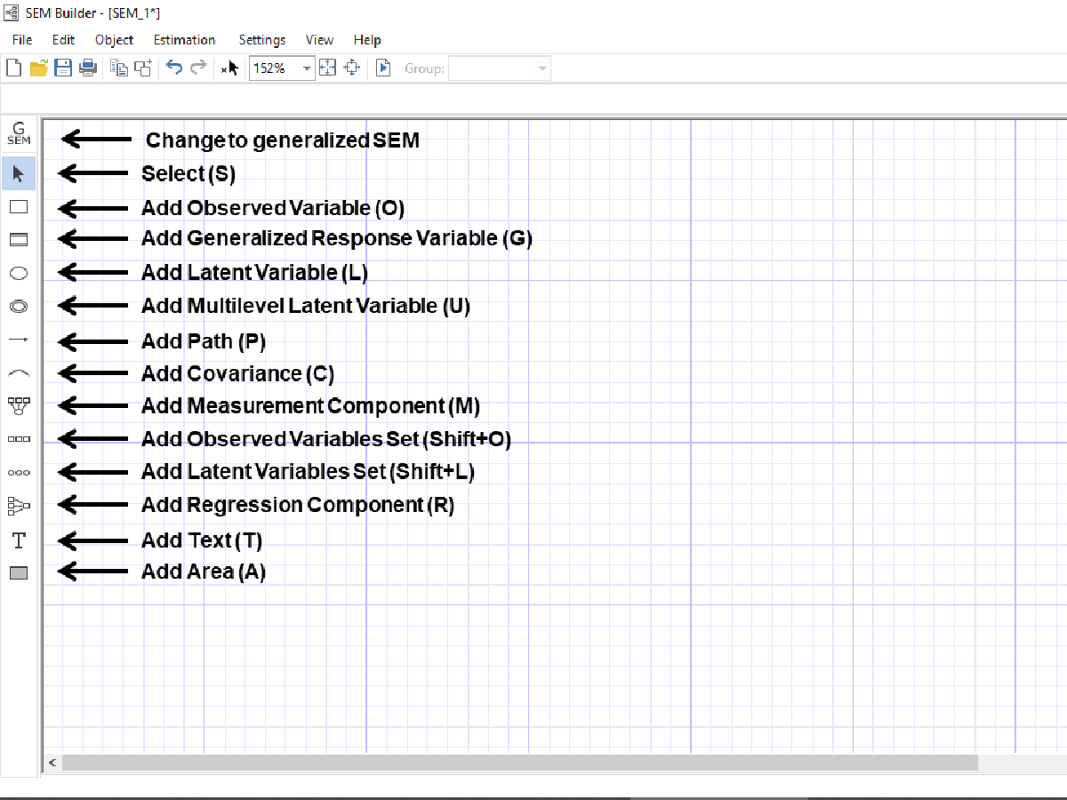
Figure 1: SEM Builder
There are three ways to fit SEMs in Stata: the sem command, the gsem command,
and through the SEM Builder. The sem command is for fitting standard
linear SEMs. It is quicker and has more features for testing and interpreting
results than gsem. The gsem command is for fitting models with generalized
responses, such as binary, count, or categorical responses, models with random
effects, and mixture models. Both sem and gsem models can be fit via path
diagrams using the SEM Builder. You can open the SEM Builder window by
typing sembuilder into the Command window. See the interface in Figure 1;
click the tools you need on the left, or type their shortcuts shown in the
parentheses. To fit gsem models, the GSEM button must first be selected.
Estimation and diagram settings can be changed using the menus at the top. The
Estimate button fits the model. Path diagrams can be saved as .stsem files
to be modified later, or can be exported to a variety of image formats (for
example see Figure 2). Although this tutorial will focus on the sem and
gsem commands, the Builder shares the same functionality. You can watch a
demonstration with the SEM Builder on the StataCorp YouTube Channel:
https://www.youtube.com/watch?v=youtube.com/watch?v=HeQcha3C8Fk
To download the datasets, do-file, and path diagrams, you can type the following
into Stata’s Command window:
. net from http://www.stata.com/users/mcain/JBDS_SEM
Clicking on the SEMtutorial link will download the materials to your current
working directory. To open the do-file with the commands we’ll be using, you can
type
. doedit SEMtutorial
Commands can either be executed from the do-file or typed into the Command
window. We’ll start by loading and exploring our first dataset. These data contain
observations on four indicators for socioeconomic status of high school students as
well as their math scores, school types (private or public), and the student-teacher
ratio of their school. Alternatively, we could have used a summary statistics dataset
containing means, variances, and correlations of the variables rather than
observations.
. use math
. codebook, compact
Variable Obs Unique Mean Min Max Label _______________________________________________________________
schtype 519 2 .61079 0 1 School type ratio 519 14 16.75723 10 28 Student-Teacher ratio math 519 42 51.72254 30 71 Math score ses1 519 5 1.982659 0 4 SES item 1 ses2 519 5 2.003854 0 4 SES item 2 ses3 519 5 2.003854 0 4 SES item 3 ses4 519 5 2.003854 0 4 SES item 4 _______________________________________________________________
2 Fitting models with the sem command
2.1 Path Analysis
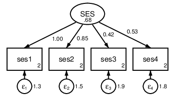
Figure 2: One-factor CFA measuring socioeconomic status (SES)
Let’s start our analysis by fitting the one-factor confirmatory factor analysis
(CFA) model shown in Figure 2. Using the sem command, paths are specified in
parentheses and the direction of the relationships are specified using arrows, i.e.
(x->y). Arrows can point in either direction, (x->y) or (y<-x). Paths can be
specified individually, or multiple paths can be specified within a single set of
parentheses, (x1 x2 x3 -> y). By default, Stata assumes that all lower-case
variables are observed and uppercase variables are latent. You can change
these settings using the nocapslatent and the latent() options. In Stata,
options are always added after a comma. We’ll see plenty of examples of this
later.
Viewing the results, we see that by default Stata constrained the first
factor loading to be 1 and estimated the variance of the latent variable. If,
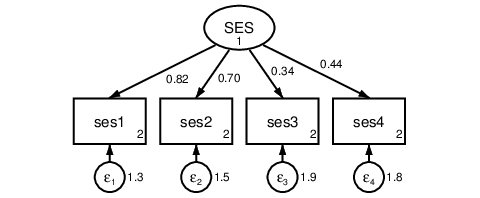
instead, we would like to constrain the variance and estimate all four factor
loadings, we could use the var() option. Constraints in any part of the model
can be specified using the @ symbol. To save room, syntax and results for
this and the remaining models will be shown on their path diagrams; see
Figure 3.
. sem (SES -> ses1-ses4), var(SES@1)
Figure 3: One-factor CFA with constrained variance.
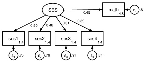
. sem (SES -> ses1-ses4 math), standardized
Figure 4: SES influences math scores.
Specifying structural paths is no different from specifying measurement paths. We
can add math score to our model and hypothesize that socioeconomic status
influences expected math performance. This model is shown in Figure 4; we’ve added
the standardized option to get standardized coefficients. With every increase of one
standard deviation in SES, math score is expected to increase by 0.45 standard
deviations.
To get fit indices for our model, we can use the postestimation command
estat gof after any sem model. Add the stats(all) option to see all fit
indices.
. estat gof, stats(all)
______________________ ______________________________________________________
Fit statistic Value Description ______________________ ______________________________________________________
Likelihood ratio chi2_ms(5) 17.689 model vs. saturated p > chi2 0.003 chi2_bs(10) 150.126 baseline vs. saturated p > chi2 0.000 ______________________ ______________________________________________________
Population error RMSEA 0.070 Root mean squared error of approximation 90% CI, lower bound 0.037 upper bound 0.107 pclose 0.147 Probability RMSEA <= 0.05 ______________________ ______________________________________________________
Information criteria AIC 11157.441 Akaike´s information criterion BIC 11221.219 Bayesian information criterion ______________________ ______________________________________________________
Baseline comparison CFI 0.909 Comparative fit index TLI 0.819 Tucker-Lewis index ______________________ ______________________________________________________
Size of residuals SRMR 0.040 Standardized root mean squared residual CD 0.532 Coefficient of determination ______________________ ______________________________________________________
Satorra-Bentler adjusted model fit indices can be obtained by adding
the vce(sbentler) option to our model statement and recalculating the
model fit indices. This option still uses maximum likelihood estimation, the
default, but adjusts the standard errors and the fit indices. Alternatively,
estimation can be changed to asymptotic distribution-free or full-information
maximum likelihood for missing values using the method(adf) or method(mlmv)
options, respectively. For this example, we’ll use the Satorra-Bentler adjustment
(Satorra & Bentler, 1994). First, we’ll store the current model to use again
later.
. estimates store m1
. sem (SES -> ses1-ses4 math), vce(sbentler)
Endogenous variables Measurement: ses1 ses2 ses3 ses4 math
______________________ ______________________________________________________
Fit statistic Value Description ______________________ ______________________________________________________
Likelihood ratio chi2_ms(5) 17.689 model vs. saturated p > chi2 0.003 chi2_bs(10) 150.126 baseline vs. saturated p > chi2 0.000 Satorra-Bentler chi2sb_ms(5) 17.804 p > chi2 0.003 chi2sb_bs(10) 153.258 p > chi2 0.000 ______________________ ______________________________________________________
Population error RMSEA 0.070 Root mean squared error of approximation 90% CI, lower bound 0.037 upper bound 0.107 pclose 0.147 Probability RMSEA <= 0.05 Satorra-Bentler RMSEA_SB 0.070 Root mean squared error of approximation ______________________ ______________________________________________________
Information criteria AIC 11157.441 Akaike´s information criterion BIC 11221.219 Bayesian information criterion ______________________ ______________________________________________________
Baseline comparison CFI 0.909 Comparative fit index TLI 0.819 Tucker-Lewis index Satorra-Bentler CFI_SB 0.911 Comparative fit index TLI_SB 0.821 Tucker-Lewis index ______________________ ______________________________________________________
Size of residuals SRMR 0.040 Standardized root mean squared residual CD 0.532 Coefficient of determination ______________________ ______________________________________________________
The SB-adjusted CFI is still rather low, 0.91, indicating poor fit. We can use
estat mindices to compute modification indices that can be used to check for paths
and covariances that could be added to the model to improve fit. First, we’ll need to
restore our original model.
The MI, df, and P>MI are the estimated chi-squared test statistic, degrees of
freedom, and $p$ value of the score test testing the statistical significance of the
constrained parameter. By default, only parameters that would significantly ($p<0.05$)
improve the model are reported. The EPC is the amount that the parameter is
expected to change if the constraint is relaxed. According to these results, we see that
there is a stronger relationship between the first and second indicator for SES than
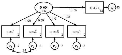
would be expected given our model, $\mathtt {MI}=16.57, p<0.001$. We could consider adding a residual covariance
between these two indicators to our model using the cov() option. We use
the e. prefix to refer to a residual variance of an endogenous variable; see
Figure 5.
. sem (SES -> ses1-ses4 math), cov(e.ses1*e.ses2)
Figure 5: CFA with residual covariance.
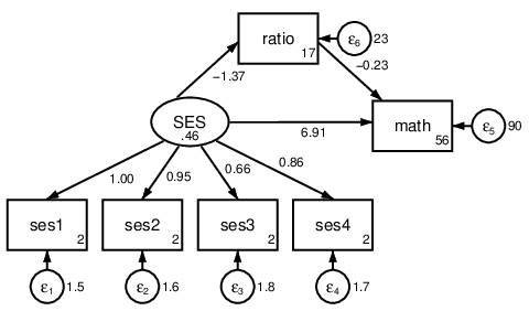
One potential explanation of the effect that SES has on math score is that
students of higher SES attend schools with smaller student to teacher ratios. We can
test this hypothesis using the mediation model shown in Figure 6. Here, we get
estimates of the direct effects between each of our variables, but what we would really
like to test is the indirect effect between SES and math through ratio. We can get
direct effects, indirect effects, and total effects of mediation models with the
postestimation command estat teffects.
. sem (SES -> ses1-ses4 ratio math) (ratio -> math)
Figure 6: Student-teacher ratio mediates the effect of SES on math score.
. estat teffects
Direct effects ______________
________________________________________________________________
OIM Coefficient std. err. z P>|z| [95% conf. interval] ______________
________________________________________________________________
Structural ratio SES -1.367306 .5562429 -2.46 0.014 -2.457522 -.2770903 ____________
________________________________________________________________
math ratio -.2256084 .1026128 -2.20 0.028 -.4267257 -.024491 SES 6.908564 1.583778 4.36 0.000 3.804417 10.01271 ______________
________________________________________________________________
Measurement ses1 SES 1 (constrained) ____________
________________________________________________________________
ses2 SES .9450302 .1643867 5.75 0.000 .6228382 1.267222 ____________
________________________________________________________________
ses3 SES .6632608 .1725434 3.84 0.000 .3250819 1.00144 ____________
________________________________________________________________
ses4 SES .8574695 .2012317 4.26 0.000 .4630625 1.251876 ______________
________________________________________________________________
Indirect effects ______________
________________________________________________________________
OIM Coefficient std. err. z P>|z| [95% conf. interval] ______________
________________________________________________________________
Structural ratio SES 0 (no path) ____________
________________________________________________________________
math ratio 0 (no path) SES .3084758 .1451257 2.13 0.034 .0240346 .5929169 ______________
________________________________________________________________
Measurement ses1 SES 0 (no path) ____________
________________________________________________________________
ses2 SES 0 (no path) ____________
________________________________________________________________
ses3 SES 0 (no path) ____________
________________________________________________________________
ses4 SES 0 (no path) ______________
________________________________________________________________
Total effects ______________
________________________________________________________________
OIM Coefficient std. err. z P>|z| [95% conf. interval] ______________
________________________________________________________________
Structural ratio SES -1.367306 .5562429 -2.46 0.014 -2.457522 -.2770903 ____________
________________________________________________________________
math ratio -.2256084 .1026128 -2.20 0.028 -.4267257 -.024491 SES 7.217039 1.599953 4.51 0.000 4.081189 10.35289 ______________
________________________________________________________________
Measurement ses1 SES 1 (constrained) ____________
________________________________________________________________
ses2 SES .9450302 .1643867 5.75 0.000 .6228382 1.267222 ____________
________________________________________________________________
ses3 SES .6632608 .1725434 3.84 0.000 .3250819 1.00144 ____________
________________________________________________________________
ses4 SES .8574695 .2012317 4.26 0.000 .4630625 1.251876 ______________
________________________________________________________________
In the second group of the output, we see that the mediation effect is not
statistically significant, $z=1.48, p=0.138$. We may consider bootstrapping this effect to get a
more powerful test. We can do this with the bootstrap command. First, we
need to get labels for the effects we would like to test. We can get these by
replaying our model results with the coeflegend option. We can use these
labels to construct an expression for the mediation effect that we’re calling
indirect. We put this expression in parentheses after bootstrap and put any
bootstrapping options after a comma; then, we put the model and its options after
a colon. Multiple expressions can be included using multiple parentheses
sets.
. sem, coeflegend
Structural equation model Number of obs = 519 Estimation method: ml
Log likelihood = -7117.1959
( 1) [ses1]SES = 1 ______________
________________________________________________________________
Coefficient Legend ______________
________________________________________________________________
Structural ratio SES -1.367306 _b[ratio:SES] _cons 16.75723 _b[ratio:_cons] ____________
________________________________________________________________
math ratio -.2256084 _b[math:ratio] SES 6.908564 _b[math:SES] _cons 55.50311 _b[math:_cons] ______________
________________________________________________________________
Measurement ses1 SES 1 _b[ses1:SES] _cons 1.982659 _b[ses1:_cons] ____________
________________________________________________________________
ses2 SES .9450302 _b[ses2:SES] _cons 2.003854 _b[ses2:_cons] ____________
________________________________________________________________
ses3 SES .6632608 _b[ses3:SES] _cons 2.003854 _b[ses3:_cons] ____________
________________________________________________________________
ses4 SES .8574695 _b[ses4:SES] _cons 2.003854 _b[ses4:_cons] ______________
________________________________________________________________
var(e.ses1) 1.541523 _b[/var(e.ses1)] var(e.ses2) 1.588663 _b[/var(e.ses2)] var(e.ses3) 1.795421 _b[/var(e.ses3)] var(e.ses4) 1.660672 _b[/var(e.ses4)] var(e.ratio) 23.41179 _b[/var(e.ratio)] var(e.math) 89.51067 _b[/var(e.math)] var(SES) .4562495 _b[/var(SES)] ______________
________________________________________________________________
LR test of model vs. saturated: chi2(8) = 21.72 Prob > chi2 = 0.0055
. bootstrap indirect=(_b[ratio:SES]*_b[math:ratio]), reps(1000) nodots: /// > sem (SES -> ses1-ses4 ratio math) (ratio -> math)
Bootstrap results Number of obs = 519 Replications = 1,000
Command: sem (SES -> ses1-ses4 ratio math) (ratio -> math) indirect: _b[ratio:SES]*_b[math:ratio]
We’ve added the reps(1000) option to compute 1,000 bootstrap replications and
the nodots option to suppress displaying a dot for each replication. To get 95
percentile confidence intervals based on our bootstrap sampling distribution, we can
follow with the postestimation command estat bootstrap using the percentile
option. The resulting confidence interval contains zero so we cannot reject the null
hypothesis.
. estat bootstrap, percentile
Bootstrap results Number of obs = 519 Replications = 1000
Command: sem (SES -> ses1-ses4 ratio math) (ratio -> math) indirect: _b[ratio:SES]*_b[math:ratio]
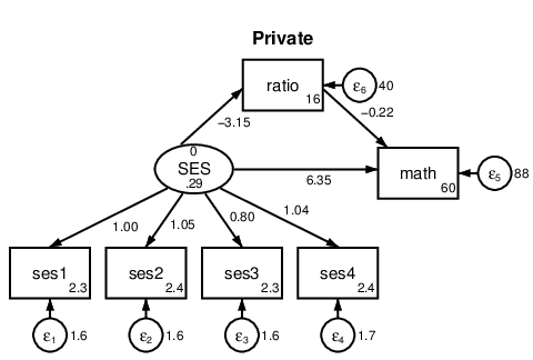
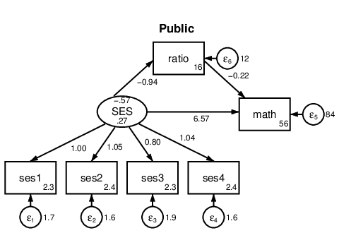
Finally, we may consider comparing our mediation across groups. Group analysis can
be done in Stata by adding the group() option. We would like to compare students
in public schools versus private schools so we will specify schtype as our
grouping variable. Then, we can use ginvariant() to specify the types of
parameters we would like to constrain across groups. All other variables
will be estimated separately for each group. The ginvariant() options are
listed in Table 1. If we don’t specify any ginvariant option, by default
Stata will constrain measurement coefficients and measurement intercepts,
ginvariant(mcoef mcons). See the model in Figure 7. Now when we run
estat teffects, we will get a separate estimated mediation effect for each
group.
. sem (SES -> ses1-ses4 math) (ratio -> math), group(schtype)
Figure 7: Group analysis.
. estat teffects, nodirect nototal compact
Indirect effects ______________
________________________________________________________________
OIM Coefficient std. err. z P>|z| [95% conf. interval] ______________
________________________________________________________________
Structural math SES Private .7043843 .4184641 1.68 0.092 -.1157902 1.524559 Public .2035724 .1710134 1.19 0.234 -.1316076 .5387525 ____________
________________________________________________________________
ratio ____________
________________________________________________________________
ses1 ____________
________________________________________________________________
ses2 ______________
________________________________________________________________
Measurement ses3 ____________
________________________________________________________________
ses4 ______________
________________________________________________________________
Table 1: ginvariant() suboptions
Option
Description
mcoef
measurement coefficients
mcons
measurement intercepts
merrvar
covariances of measurement errors
scoef
structural coefficients
scons
structural intercepts
serrvar
covariances of structural errors
smerrcov
covariances between structural and measurement errors
meanex
means of exogenous variables
covex
covariances of exogenous variables
all
all the above
none
none of the above
To test whether these mediation effects significantly differ, we can conduct a Wald
test with the test or testnl postestimation commands, again using the labels from
the coeflegend option. Because mediation effects are nonlinear, we will use
testnl. The mediation effects do not significantly differ between groups,
$\chi ^2(1)=1.27,p=0.260$.
To test group differences in each direct path, we can use the postestimation
command estat ginvariant. These results show us Wald tests evaluating
constraining parameters that were allowed to vary across groups and score tests
evaluating relaxing constraints. Both are testing whether individual paths
significantly differ across groups.
2.3 Growth Curve Modeling
The last model we will fit using sem is a growth curve model. This will require a new
dataset.
. use crime
. describe
Contains data from crime.dta Observations: 359 Variables: 4 4 Oct 2012 16:22 (_dta has notes) _______________________________________________________________
Variable Storage Display Value name type format label Variable label _______________________________________________________________
lncrime0 float %9.0g ln(crime rate) in Jan & Feb lncrime1 float %9.0g ln(crime rate) in Mar & Apr lncrime2 float %9.0g ln(crime rate) in May & Jun lncrime3 float %9.0g ln(crime rate) in Jul & Aug _______________________________________________________________
Sorted by:
These data are from Bollen and Curran (2006); they contain crime rates collected
in two-month intervals for the first eight months of 1995 for 359 communities in New
York state. We would like to fit a linear growth curve to these data to model how
crime rate changed over time. In our model, we can set constraints using the @ symbol
as we did before. To constrain all intercepts to 0, we can add the nocons option. We
will also need the means() option. By default, Stata constrains the means of latent
variables to 0. For this model, we would like to estimate them so we need
to specify the latent variable names inside means(). We may also consider
constraining all the residual variances to equality by constraining each of
them to the same arbitrary letter or word, in this case eps. See the model in
Figure 8.
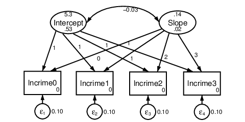
The estimated mean log crime rate at the beginning of the study was 5.33 and it
increased by an average of 0.14 every two months. We could have fit this same model
using gsem. One way we can do this is to simply replace sem with gsem in the
command in Figure 8. Alternatively, we can can think of this as a multilevel
model, and fit it using gsem’s notation for random effects. Let’s do that
next.
3 Fitting models with the gsem command
3.1 Models with Random Effects
The gsem command implements generalizations to the standard linear structural
equation model implemented in sem, such as models with generalized-linear response
variables, random effects, and categorical latent variables (latent classes). Its syntax is
the same as sem, with some different options and postestimation commands. We will
start by fitting a random-slope model to the crimes dataset, reproducing the
results we obtained with the growth curve model using sem. First, we need to
create an observation identification variable and reshape the data into long
format.
Data Wide -> Long _____________________________________________________________________________
Number of observations 359 -> 1,436 Number of variables 5 -> 3 j variable (4 values) -> time xij variables: lncrime0 lncrime1 ... lncrime3 -> lncrime _____________________________________________________________________________
. summarize
Variable Obs Mean Std. dev. Min Max ______________ _________________________________________________________
id 1,436 180 103.6701 1 359 time 1,436 1.5 1.118423 0 3 lncrime 1,436 5.551958 .7856259 2.415164 9.575166
We now have long-format data in which we have several rows of observations for
each individual; we’re ready to fit our random-slope model. We specify random effects
in gsem by adding brackets enclosing the clustering variable to the latent variable, i.e.
Intercept[id]. This tells Stata to include a latent variable in the model called
Intercept that has variability at the id level. As with other latent variables, it will
have a mean of 0 and an initial factor loading of 1, so the only parameter
this term introduces is a level-2 variance. Random coefficients can be added
to any term by interacting a latent random effect with that variable, i.e.
c.time#Slope[id].
Interactions in Stata are specified using #; interaction terms are assumed to be
factor variables unless prefixed by c. to indicate that they are continuous variables.
Contrarily, main-effect terms are assumed to be continuous unless prefixed by i. to
indicate that they are factor variables. We’ll see this in the next example. This factor
variable notation is not available using sem.
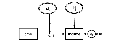
See the syntax and results of the random slope model in Figure 9; these results
replicate those by sem. In the SEM Builder, random effects are represented as
double-bordered ovals labeled with the clustering variable to indicate that they
represent variability at the cluster level.
. gsem (Intercept[id] time c.time#Slope[id] -> lncrime)
Figure 9: Random-slope model on crime rate.
3.2 Models with Generalized Responses
The gsem command can also be used to fit generalized linear SEMs; that is, SEMs in
which an endogenous variable is distributed according to some distribution family and
is related to the linear prediction of the model through a link function. See Table 2
for a list of available distribution families and links. Either the family and link can be
specified, i.e. family(bernoulli) link(logit), or some combinations have
shortcuts that you can specify instead, i.e. logit. For this example, we will return to
the first dataset.
Table 2: gsem distribution families and link functions
family() options
link() options
identity
log
logit
probit
cloglog
gaussian
X
X
bernoulli
logit
probit
cloglog
beta
X
X
X
binomial
X
X
X
ordinal
ologit
oprobit
ocloglog
multinomial
mlogit
Poisson
poisson
negative binomial
nbreg
exponential
exponential
Weibull
weibull
gamma
gamma
loglogistic
loglogistic
lognormal
lognormal
Note: X indicates possible combinations. Where applicable, regression names that
imply that family/link combination are shown. If no family/link are provided,
family(gaussian) link(identity) is assumed.
. use math
. codebook, compact
Variable Obs Unique Mean Min Max Label _______________________________________________________________
schtype 519 2 .61079 0 1 School type ratio 519 14 16.75723 10 28 Student-Teacher ratio math 519 42 51.72254 30 71 Math score ses1 519 5 1.982659 0 4 SES item 1 ses2 519 5 2.003854 0 4 SES item 2 ses3 519 5 2.003854 0 4 SES item 3 ses4 519 5 2.003854 0 4 SES item 4 _______________________________________________________________
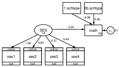
In our previous analysis, we had treated each socioeconomic status Likert item as
continuous. Now, we will treat them as ordinal using gsem. Adding the ologit option
will fit the measurement model using the ordinal family with a logistic link. We will
also use factor variable notation to include indicator variables for school type in our
analysis. See figure Figure 10. By adding schtype as a factor variable, a
dummy variable for each level of schtype is included in the model. The path
coefficient for the base level, by default the lowest, is constrained to zero. To get
exponentiated coefficients, we can follow with the postestimation command estateform.
. sem (SES -> ses1-ses4, ologit) (SES i.schtype -> math)
Figure 10: Ordinal logistic regression model.
. estat eform ses1 ses2 ses3 ses4 ______________
________________________________________________________________
exp(b) Std. err. z P>|z| [95% conf. interval] ______________
________________________________________________________________
ses1 SES 2.718282 (constrained) ______________
________________________________________________________________
ses2 SES 2.311549 .483485 4.01 0.000 1.534141 3.482899 ______________
________________________________________________________________
ses3 SES 1.449492 .180061 2.99 0.003 1.136257 1.849077 ______________
________________________________________________________________
ses4 SES 1.628133 .2474222 3.21 0.001 1.208748 2.193029 ______________
________________________________________________________________
4 Conclusion
In this tutorial, we’ve shown the basics of fitting SEMs in Stata using the sem and
gsem commands, and have provided example datasets and syntax online to follow
along. We demonstrated confirmatory factor analysis, mediation, group analysis,
growth curve modeling, and models with random effects and generalized responses.
However, there are many possibilities and options not included in this tutorial, such
as latent class analysis models, nonrecursive models, reliability models, mediation
models with generalized responses, multivariate random-effects models, and much
more. Visit Stata’s documentation to see all the available options for these
commands, their methods and formulas, and many more examples online at
https://www.stata.com/manuals/sem.pdf.
References
Bollen, K. A., & Curran, P. J.
(2006). Latent curve models: A structural equation perspective (Vol. 467).
John Wiley & Sons.
Satorra, A., & Bentler, P. M.
(1994). Corrections to test statistics and standard errors in covariance
structure analysis. In Latent variables analysis: Applications for developmentalresearch. (pp. 399–419). Sage Publications, Inc.
StataCorp.
(2021). Stata statistical software: Release 17. StataCorp LLC.