Keywords: Model selection criterion · Bayesian estimation · Latent growth models · Missing data · Robust method
Bayesian approach is becoming increasingly important in estimating models as it provides many advantages in dealing with complex data (e.g., Dunson, 2000). However, there is no well-defined model selection criterion or index in a Bayesian context (e.g., Celeux, Forbes, Robert, & Titterington, 2006). It is due to at least three problems. First, in a Bayesian context there are two versions of deviance because the Bayesian procedure generates Monte Carlo Markov chains for each parameter. One version is the posterior estimate, which can be estimated by a function of an estimate of a parameter. Another version is the Monte Carlo estimate of the expected deviance based on Bayesian iterations, which can be estimated as the posterior mean of a converged Markov chain. In short, the former is the deviance of the averaged estimates, and the latter is the average of all deviance iterations. The second problem is related to the complexity of the raw data. The data often come from heterogeneous populations which almost unavoidable contain outliers and missing values. The estimates from mis-specified models may result in severely misleading conclusions. The third problem relates to the likelihood function. When latent variables are considered in statistical models, the likelihood function can be an observed-data likelihood function, a complete-data likelihood function, or a conditional likelihood function (Celeux et al., 2006). Furthermore, if data come from heterogeneous populations, the class membership indicator may have different versions, for example, a posterior mode or a posterior mean. Also, with missing data, the likelihood functions have different ways to construct.
Traditional model selection criteria or indices are available for researchers who try to select the best-fit model from a large set of candidate models. Akaike (1974) proposed the Akaike’s information criterion (AIC), which offers a relative measure of the information lost. For Bayesian models the Bayes factor, which is the ratio of posterior odds to prior odds, can work for both hypothesis testing and model comparison. But the Bayes factor is often difficult or impossible to calculate, especially for models that involve random effects, large numbers of unknowns or improper priors. To approximate the Bayes factor, Schwarz (1978) developed the Bayesian information criterion (BIC, sometimes called the Schwarz criterion). To obtain more precise indices, Bozdogan (1987) proposed the consistent Akaike information criterion (CAlC), and Sclove (1987) proposed the sample-size adjusted Bayesian information criterion (ssBIC). The deviance information criterion (DIC; Spiegelhalter, Best, Carlin, & Linde, 2002) is a recently developed criterion designed for hierarchical models. It is based on the posterior distribution of the log-likelihood and is useful in Bayesian model selection problems where the posterior distributions have been obtained by Markov chain Monte Carlo (MCMC) simulation. DIC is usually regarded as a generalization of AIC and BIC. It is defined analogously to AIC or BIC with a penalty term of the number equal to effective model parameters in Bayesian models. In practice, rough DIC (RDIC or DICV in some literature, e.g., Oldmeadow & Keith, 2011) is an approximation of DIC. The mathematical forms of AIC, BIC, CAIC, ssBIC, and DIC are closely related to each other. They all try to find a balance between the accuracy and the complexity of the fitting model. For all indices above, the model with a smaller criterion/index value is better supported by data.
Lu, Zhang, and Cohen (2013) proposed a series of Bayesian model selection indices based on the traditional ones. However, in Lu et al. (2013) the performances of these indices were investigated when data were non-mixture, normally distributed, and with simple non-ignorable missingness. And only latent growth models were used.
To address the challenges in model selection criterion/index in a Bayesian context, this paper proposes ten model selection indices. This paper also examines the performance of these indices under various conditions by conducting five simulation studies to cover different latent growth models, such as the robust growth models for non-normally distributed data, robust growth mixture models, and the extended robust growth mixture models with missing values. We consider latent growth models because they are very flexible in modeling complex data and becoming increasingly popular in statistical, psychological, behavioral, and educational areas.
The rest of the article consists of five sections. Section 2 presents and formulates three types of models we used in this paper: latent growth models (including growth curve models, growth mixture models, and extended growth mixture models), robust growth models (including three types of robust models), and models that account for missingness (we focus on non-ignorable missingness). Section 3 proposes ten model selection indices in the framework of Bayesian growth models with missing data. Section 4 conducts five simulation studies to evaluate the performance of the Bayesian indices. Model selection results are analyzed, summarized, and compared. Section 5 illustrates the application of these model selection indices in real data analysis. Section 6 discusses the implications and future directions of this study.
Our investigation of the performance of the Bayesian selection indices involves fitting growth models to complex data. In this section, different types of growth models are briefly introduced. Given the fact that the data used in growth models are almost inevitably contain attrition (e.g., Little & Rubin, 2002; Lu, Zhang, & Lubke, 2011; Yuan & Lu, 2008) and outliers (e.g., Maronna, Martin, & Yohai, 2006), different types of growth models are developed, which include traditional latent growth curve models with missing data (Lu et al., 2013), robust growth curve models (Zhang, Lai, Lu, & Tong, 2013) with missing data (Lu & Zhang, 2021), growth mixture models (e.g., Bartholomew & Knott, 1999) with missing data (Lu & Zhang, 2014), extended growth mixture models (EGMMs, Muthén & Shedden, 1999) with missing data (Lu & Zhang, 2014), and robust growth mixture models with missing data (Lu & Zhang, 2014).
In the following, we discuss three types of models: latent growth models (including growth curve models, growth mixture models, and extended growth mixture models), robust growth models (including three types of robust models), and models that account for missingness (we focus on non-ignorable missingness). By combining different elements of these models, it becomes possible to consider a series of growth models with a variety of missing data mechanisms and contaminated data.
The mathematical form of a latent growth curve model is
| (1) |
where $\by _{i}$ is a $T\times 1$ vector of outcomes for participant $i \, (i=1,...,N)$, $\boldeta _{i}$ is a $q\times 1$ vector of latent effects, $\bLambda $ is a $T\times q$ matrix of factor loadings for $\boldeta _{i}$, $\be _{i}$ is a $T\times 1$ vector of residual or measurement errors, $\bbeta $ is a $q\times 1$ vector of fixed-effects, and $\bxi _{i}$ captures the variation of $\boldeta _{i}$. We have to note that $\be _{i}$ and $\bxi _{i}$ are usually assumed normally distributed but not necessary. When data have outliers and are heavy-tailed, this assumption might cause estimate biases. To reduce the effects of outliers, we consider robust models in this study.
A growth mixture model can be expressed as
| (2) |
where $\pi _{k}$ is the invariant class probability (or weight) for class $k$ satisfying $0\leq \pi _{k}\leq 1$ and $\sum _{k=1}^K \pi _{k}=1$ (e.g., McLachlan & Peel, 2000), and $f_{_{k}}(\by _{i}) (k=1,\ldots , K)$ is the density of a latent growth model for class $k$.
For extended growth mixture models (EGMMs, Muthén & Shedden, 1999), $\pi _{k}$ is not invariant across individuals. It is allowed to vary individually depending on covariates, so it is expressed as $\pi _{ik}(\bx _i)$. If a probit link function is used, then
| (3) |
where $\Phi (\cdot )$ is the cumulative distribution function (CDF) of the standard normal distribution, and $X_{i}=(1, \bx _{i}')'$ with an $r\times 1$ vector of observed covariates $\bx _{i}$. Note that $\Phi (X_{i}' \, \bvarphi _{k})=\sum _{j=1}^k \pi _{ij}(\bx _i)$ and $\Phi (X_{i}' \, \bvarphi _{K}) \equiv 1$.
A dummy variable $\bz _{i}=(z_{i1},z_{i2},...,z_{iK})'$ is used to indicate the class membership. If individual $i$ comes from group $k$, $z_{ik}=1$ and $z_{ij}=0$ $(\forall j\neq k)$. $\bz _{i}$ is multinomially distributed (McLachlan & Peel, 2000, p.7), that is, $\bz _{i} \sim MultiNomial(\pi _{i1},\pi _{i2},...,\pi _{iK})$.
When data have outliers and are heavy-tailed, robust methods are used to reduce the effects of outliers. As t-distributions are more robust than normal distributions, the following are robust growth models (Lu & Zhang, 2021; Zhang et al., 2013).
(1) t-Normal (TN) model in which the measurement errors are t-distributed and the latent random effects are normally distributed,
| (4) |
where $Mt_{T}(\textbf {0}, \bTheta , \nu )$ is a $T$-dimensional multivariate t-distribution with a scale matrix $\bTheta $ and degrees of freedom $\nu $, and $MN_{q}(\textbf {0}, \bPsi )$ is a $q$-dimensional multivariate Normal distribution with a covariance matrix $\bPsi $.
(2) Normal-t (NT) model in which the measurement errors are normally distributed but the latent random effects are t-distributed,
| (5) |
(3) t-t (TT) model in which both the measurement errors and the latent random effects are t-distributed,
| (6) |
We focus on the non-ignorable missingness in this paper. To build models with non-ignorable missingness, selection models (Glynn, Laird, & Rubin, 1986; Little, 1993, 1995) are used. For individual $i$, let $\boldm _{i}=(m_{i1},m_{i2},...,m_{iT})'$ be a missing data indicator for $\by _{i}$, with $m_{it}=1$ when $y_{it}$ is missing and $0$ when observed. Let $\tau _{it}=p(m_{it}=1)$ be the probability that $y_{it}$ is missing. Then $m_{it}\sim \textrm {Bernoulli}(\tau _{it})$, so its density function is $f(m_{it})=\tau _{it}^{m_{it}}(1-\tau _{it})^{(1-m_{it})}$. The missingness probability $\tau _{it}$ can have different forms. Lu and Zhang (2014) proposed the following non-ignorable missingness mechanisms for mixture models.
(1) Latent-Class-Intercept-Dependent (LCID) missingness in which $\tau _{it}$ is a function of latent class, covariates, and latent individual initial levels. For example, students are more likely to miss a test if their starting levels of that course are low. We model it as follows:
where $I_{i}$ is the latent initial levels for individual $i$, $\gamma _{It}$ is the coefficient for $I_{i}$, $\bgamma _{zt}$ is the coefficient for class membership, and $\bgamma _{xt}$ are coefficients for covariates. For non-mixture homogenous growth models, LCID can be simplified to Latent-Intercept-Dependent (LID) without the class membership indicator $\bz _{i}$ and expressed as $\tau _{it} = \Phi (\gamma _{0t} + I_{i}\gamma _{It} + \bx _{i}'\bgamma _{xt})$, where $\gamma _{0t}$ is the intercept.
(2) Latent-Class-Slope-Dependent (LCSD) missingness in which $\tau _{it}$ is a function of latent class, covariates, and latent individual slopes of growth. For example, students are more likely to miss a test if they have slow growth of the course. In this case, $\tau _{it}$ can be modeled as
where $S_{i}$ is the latent slope for individual $i$, and $\gamma _{St}$ is the coefficient for $S_{i}$. Similarly, for non-mixture homogeneous growth models, LCSD is simplified to Latent-Slope-Dependent (LSD) case as $\tau _{it} =\Phi (\gamma _{0t} + S_{i}\gamma _{St} + \bx _{i}'\bgamma _{xt})$.
(3) Latent-Class-Outcome-Dependent (LCOD) missingness in which $\tau _{it}$ is a function of latent class, covariates, and potential outcomes that may be missing. For example, a student who feels he is not doing well on the test may be more likely to give up taking the rest of the test. We express $\tau _{it}$ as
where $y_{it}$ is the potential outcomes for individual $i$ at time $t$, and $\gamma _{yt}$ is the coefficient for $y_{it}$. And LCOD can be simplified to Latent-Outcome-Dependent (LOD) for non-mixture homogeneous growth models with a probability of missingness $\tau _{it} =\Phi (\gamma _{0t} + y_{it} \gamma _{yt}+\bx _{i}'\bgamma _{xt})$.
In a more general framework, LCID and LCSD can be further encompassed into Latent-Class-Random Effect-Dependent missingness as intercept and slope are different random effects according to different situations under consideration. And for non-mixture structure, LID and LSD are encompassed into Latent-Random Effect-Dependent missingness.
In this section, we propose ten model selection criteria in the framework of Bayesian growth models with missing data. The definitions of the selection criteria are listed in Table 1. The model selection criteria in the table are based on two versions of deviance in the Bayesian context, $E_{D|y}[D(\theta )]$ and $D(E_{\theta |y}[\theta ])$. As we have discussed in the introduction section, $E_{\theta |y}[D]$ is the expected value of all the deviances, and $D(E_{\theta |y}[\theta ])$ is the deviance score based on the expected parameters. For different models, the detailed mathematical forms of these two deviances are different. In this paper, we focus on both homogeneous and heterogeneous latent growth models with non-ignorable missing data.
| Index = | Deviance + | Penalty |
| Dbar.AIC$^1$ | $\overline {D(\theta )}^4$ | 2 p |
| Dbar.BIC$^2$ | $\overline {D(\theta )}$ | log(N) p |
| Dbar.CAIC | $\overline {D(\theta )}$ | (log(N)+1) p |
| Dbar.ssBIC | $\overline {D(\theta )}$ | log((N+2)/24) p |
| RDIC | $\overline {D(\theta )}$ | var(Dbar)/2 |
| Dhat.AIC | $D(\hat {\theta })^5$ | 2 p |
| Dhat.BIC | $D(\hat {\theta })$ | log(N) p |
| Dhat.CAIC | $D(\hat {\theta })$ | (log(N)+1) p |
| Dhat.ssBIC | $D(\hat {\theta })$ | log((N+2)/24) p |
| DIC$^3$ | $D(\hat {\theta })$ | 2 pD |
Note.
1. $p$ is the number of parameters.
2. $N$ is the sample size.
3. $pD=\overline {D(\theta )}-D(\hat {\theta })$.
4. $\overline {D(\theta )}$ is shown as in eqn.(10) for growth curve models and as in eqn.(13) for growth mixture models.
5. $D(\hat {\theta })$ is shown as in eqn.(12) for growth curve models and as in eqn.(14) for growth mixture models.
We first look at the homogeneous growth curve models with non-ignorable missing data. One version of deviance, $E_{D|y}[D(\theta )]$, is approximated by
where $S$ is the number of iterations for converged Markov chains, $l_{it}^{(s)}(\theta |y,m)$ = $log(L_{it}^{(s)}(\theta |y,m))$ is a conditional joint loglikelihood function (see, Celeux et al., 2006) of $y$ and $m$, $m_{it}$ is the missing data indicator for individual $i$ at time $t$ with a likelihood function $l_{ikt}(m) = m_{it}log(\tau _{it})+(1-m_{it})log (1-\tau _{it})$, where $\tau _{it}$ is the missing data rate for individual $i$ at time $t$ and is defined differently for different missingness models as in the previous section. When $y_{it}$ is missing, the corresponding likelihood is excluded. So combining $y$ and $m$, the conditional likelihood function of a selection model with non-ignorable missing data can be expressed as
And the other version of deviance, $D(E_{\theta |y}[\theta ])$, is approximated by
where $\hat {\theta }$ is the posterior mean of parameter estimates across $S$ iterations.
For growth mixture models with missing data, $E_{\theta |y}[D]$ is expressed as
where $\bz _{i}=(z_{i1},z_{i2},...,z_{iK})$ is the class membership indicator which follows a multinomial distribution, $\bz _{i} \sim MultiNomial(\pi _{i1},\pi _{i2},...,\pi _{iK})$, and $z_{ik}^{(s)}$ is the class membership estimated at iteration $s$. And
where $\hat {z}_{ik}$ is the posterior mode of class membership, $\hat {\theta }$ is the posterior mean of parameter estimates across all $S$ iterations. In both $\overline {D(\theta )}$ and $D(\hat {\theta })$ definitions of deviance, $l_{ikt}(y)$ and $l_{ikt}(m)$ are the conditional loglikelihood functions for $y_{it}$ and $m_{it}$, respectively, for individual $i$ in class $k$ at time $t$.
The difference between $\overline {D(\theta )}$ and $D(\hat {\theta })$ can be quantified by a statistic called pD (Spiegelhalter et al., 2002),
| (15) |
Based on the Jensen’s inequality (Casella & George, 1992), when $D(\theta )$ is convex, then $\overline {D(\theta )} \geq D(\hat {\theta })$ and as a result pD is positive. When $D(\theta )$ is concave, then $\overline {D(\theta )} \leq D(\hat {\theta })$ and pD is negative.
In this section, five simulation studies are conducted to evaluate the performance of the Bayesian indices. For each study, four waves of complete data are generated first and then missing data are created on each occasion according to pre-designed missing data rates. After data are generated, full Bayesian methods are used by adopting uninformative priors, obtaining conditional posterior distributions through application of a data augmentation algorithm, generating Markov chains through a Gibbs sampling procedure, conducting convergence testing, and making statistical inference for model parameters. For all simulations, the software OpenBUGS is used for the implementation of Gibbs sampling, and R is used for data-generation, convergence testing, and parameter estimation.
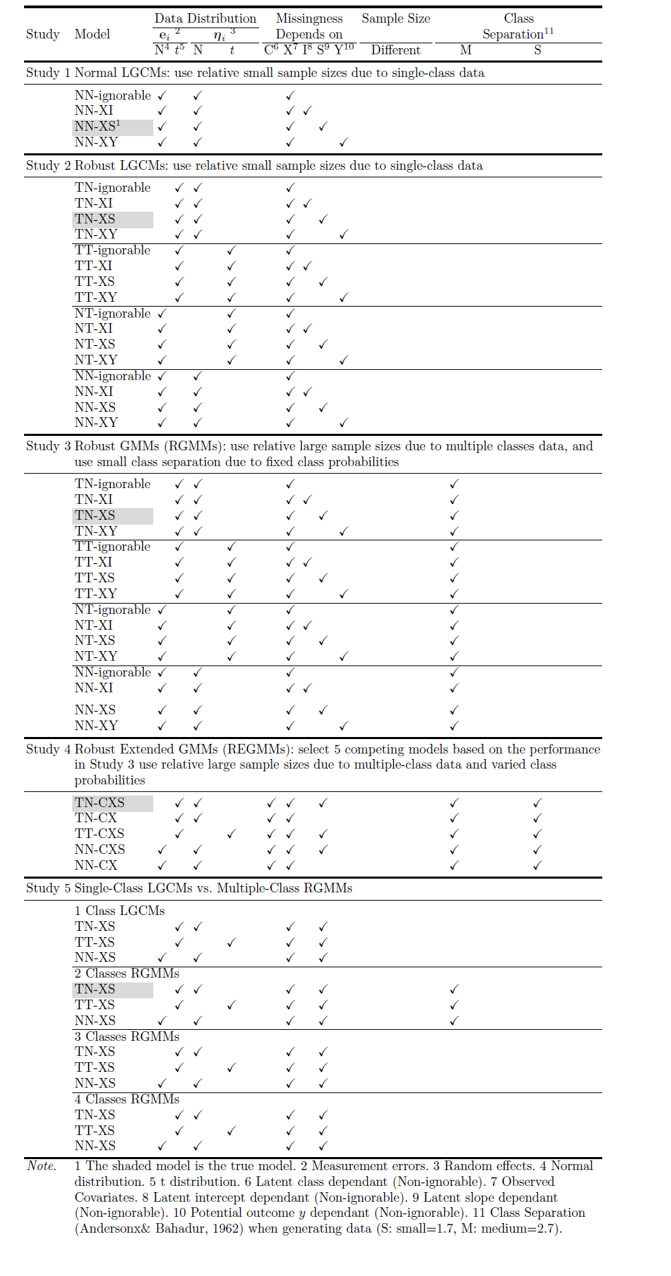
The five studies are designed such that the data complexity increases from study 1 to study 5. Studies 1-2 focus on non-mixture growth data and thus, latent growth curve models with missing data are used. Studies 3-5 focus on mixture growth data and thus, growth mixture models with missing data are used. Simulation factors include measurement error distributions, random-effects distributions, missingness patterns, sample size, and class separation (Anderson & Bahadur, 1962). Under each condition, 100 converged replications are used to calculate the model selection proportion. Table 2 lists the design details.
Study 1 investigated the performance of the Bayesian indices when data were non-mixture, homogeneous, normally distributed with non-ignorable missingness. The true model was NN-XS, which was the model with normally distributed measurement errors ($\be _{i}$) at level 1 and random effects ($\bxi _i$) at level 2, with missingness depending on covariate $x$ and latent slope $S$. Specifically, $\be _{i} \sim MN(\textbf {0}, \bI )$, $\boldeta _{i} \sim MN_{q}(\bbeta ,\bPsi )$ where $\bbeta =\textrm {(Intercept, Slope)}=(1,3)$ and $\bPsi $ was a 2 by 2 symmetric matrix with $Var(I)=1$, $Cov(I,S)=0$, and $Var(S)=4$. For missingness, the bigger the latent slope was, the higher the missing data rate would be. The missingness probit coefficients were set as $\gamma _0=(-1,-1,-1,-1)$, $\gamma _x=(-1.5,-1.5,-1.5,-1.5)$, and $\gamma _S=(0.5,0.5,0.5,0.5)$. For example, if a participant had a latent growth slope 3, with a covariate value 1, then his or her missing probability at each wave was $\tau \approx 16\%$; if the slope was 5, with the same covariate value, the missing probability increased to $\tau =50\%$; but if the slope was 1, then the missing probability decreased to $\tau =2.3\%$. The covariate $x$ was also generated from a normal distribution, $x \sim N(1, sd=0.2)$. In study 1, in total there were 16 conditions with 4 missingness mechanisms (XS non-ignorable, XY non-ignorable, XI non-ignorable, and ignorable) combined with 4 levels of sample size (1000, 500, 300, and 200). Table 3 lists the model selection proportions across 100 replications for each of these indices across all conditions in study 1. The largest proportion across 4 missingness models is indicated in the shaded cell for each index. When sample size is relatively large, 1000 or 500, all of the model selection indices, except for the rough DIC (RDIC), correctly identify the true model with 100%. When sample size becomes smaller, 300 or 200, except for the RDIC, all of the model selection indices choose the true model with certainty above 93%. Comparing the indices defined based on Dbar with those defined based on Dhat, one can see that the former performs a little bit better.
| N=1000 | N=500
| ||||||||
| Non-ignorable | Ignorable | Non-ignorable | Ignorable | ||||||
| Criteron$^1$ | NN-XS$^2$ | NN-XY$^3$ | NN-XI$^4$ | NN$^5$ | NN-XS | NN-XY | NN-XI | NN | |
| Dbar.AIC | 1$^6$ | 0.000 | 0.000 | 0.000 | 1 | 0.000 | 0.000 | 0.000 | |
| Dbar.BIC | 1 | 0.000 | 0.000 | 0.000 | 1 | 0.000 | 0.000 | 0.000 | |
| Dbar.CAIC | 1 | 0.000 | 0.000 | 0.000 | 1 | 0.000 | 0.000 | 0.000 | |
| Dbar.ssBIC | 1 | 0.000 | 0.000 | 0.000 | 1 | 0.000 | 0.000 | 0.000 | |
| RDIC | 0.013 | 0.000 | 0.987 | 0.000 | 0.038 | 0.000 | 0.962 | 0.000 | |
| Dhat.AIC | 1 | 0.000 | 0.000 | 0.000 | 1 | 0.000 | 0.000 | 0.000 | |
| Dhat.BIC | 1 | 0.000 | 0.000 | 0.000 | 1 | 0.000 | 0.000 | 0.000 | |
| Dhat.CAIC | 1 | 0.000 | 0.000 | 0.000 | 1 | 0.000 | 0.000 | 0.000 | |
| Dhat.ssBIC | 1 | 0.000 | 0.000 | 0.000 | 1 | 0.000 | 0.000 | 0.000 | |
| DIC | 1 | 0.000 | 0.000 | 0.000 | 1 | 0.000 | 0.000 | 0.000 | |
| N=300 | N=200
| ||||||||
| Dbar.AIC | 0.98125 | 0.01875 | 0.000 | 0.000 | 0.975 | 0.025 | 0.000 | 0.000 | |
| Dbar.BIC | 0.98125 | 0.01875 | 0.000 | 0.000 | 0.975 | 0.025 | 0.000 | 0.000 | |
| Dbar.CAIC | 0.98125 | 0.01875 | 0.000 | 0.000 | 0.975 | 0.025 | 0.000 | 0.000 | |
| Dbar.ssBIC | 0.98125 | 0.01875 | 0.000 | 0.000 | 0.975 | 0.025 | 0.000 | 0.000 | |
| Rough DIC | 0.1125 | 0.000 | 0.8875 | 0.000 | 0.2 | 0.03125 | 0.76875 | 0.000 | |
| Dhat.AIC | 0.95 | 0.05 | 0.000 | 0.000 | 0.9375 | 0.06875 | 0.000 | 0.000 | |
| Dhat.BIC | 0.95 | 0.05 | 0.000 | 0.000 | 0.9375 | 0.06875 | 0.000 | 0.000 | |
| Dhat.CAIC | 0.95 | 0.05 | 0.000 | 0.000 | 0.9375 | 0.06875 | 0.000 | 0.000 | |
| Dhat.ssBIC | 0.95 | 0.05 | 0.000 | 0.000 | 0.9375 | 0.06875 | 0.000 | 0.000 | |
| DIC | 1 | 0.000 | 0.000 | 0.000 | 0.98125 | 0.0125 | 0.00625 | 0.000 | |
1. The definition of each index is given in Table 1.
2. The shaded model is the true model. The model is
normal-distribution-based with
latent-slope-dependent missingness.
3. The model is normal-distribution-based with potential-outcome-dependent missingness.
4. The model is normal-distribution-based with latent-intercept-dependent missingness.
5. The model is normal-distribution-based with ignorable missingness.
6. The shaded cell has the largest proportion.
Study 2 investigated the performance of these indices when data were non-mixture homogeneous with outliers and non-ignorable missingness. The main difference between study 2 and 1 was that the data for study 2 contain outliers such that they are not normally distributed. So robust growth curve models were used. The true model was TN-XS, which means measurement errors ($\be _i$) at level 1 followed a t-distribution. Specifically, $\be _{i}$ were generated from a $t$ distribution with 5 degrees of freedom and a scale matrix $\bI $, i.e., $\be _{i} \sim Mt(\textbf {0}, \bI , 5)$. Other settings were kept the same as those in study 1. In this study, totally 32 conditions were considered with 4 data distributions (NN, TN, NT, and TT), 4 missingness patterns (XS non-ignorable, XY non-ignorable, XI non-ignorable, and ignorable), and 2 levels of sample size (1000 and 500). Table 4 lists the model selection proportions. The largest proportion across 16 missingness models is indicated in the shaded cells for each index. Except for the RDIC, all of the model selection indices correctly identify the true model. TT-XS is a competing model, which also gains high selection probabilities. This is because the normal distribution is almost identical to a t-distribution with large degrees of freedom. The degrees of freedom of t is also estimated by the model. Also, the Dbar-based indices performs a little bit better than the Dhat-based indices. Among them, Dbar-based BIC and CAIC perform best.
| N=1000 | N=500
| |||||||||
| Non-ignorable | Ignorable | Non-ignorable | Ignorable | |||||||
| Index | XS$^5$ | XY | XI | XS | XY | XI | ||||
| Dbar.AIC | TN$^1$ | 0.519 | 0.000 | 0.000 | 0.000 | 0.597 | 0.013 | 0.000 | 0.000 | |
| TT$^2$ | 0.469 | 0.000 | 0.000 | 0.012 | 0.377 | 0.000 | 0.000 | 0.000 | ||
| NT$^3$ | 0.000 | 0.000 | 0.000 | 0.000 | 0.006 | 0.000 | 0.000 | 0.000 | ||
| NN$^4$ | 0.000 | 0.000 | 0.000 | 0.000 | 0.006 | 0.000 | 0.000 | 0.000 | ||
| Dbar.BIC | TN | 0.781 | 0.000 | 0.000 | 0.000 | 0.855 | 0.013 | 0.000 | 0.000 | |
| TT | 0.200 | 0.000 | 0.000 | 0.019 | 0.113 | 0.000 | 0.000 | 0.000 | ||
| NT | 0.000 | 0.000 | 0.000 | 0.000 | 0.006 | 0.000 | 0.000 | 0.000 | ||
| NN | 0.000 | 0.000 | 0.000 | 0.000 | 0.013 | 0.000 | 0.000 | 0.000 | ||
| Dbar.CAIC | TN | 0.819 | 0.000 | 0.000 | 0.000 | 0.888 | 0.012 | 0.000 | 0.000 | |
| TT | 0.162 | 0.000 | 0.000 | 0.019 | 0.075 | 0.000 | 0.000 | 0.000 | ||
| NT | 0.000 | 0.000 | 0.000 | 0.000 | 0.000 | 0.000 | 0.000 | 0.000 | ||
| NN | 0.000 | 0.000 | 0.000 | 0.000 | 0.019 | 0.000 | 0.000 | 0.000 | ||
| Dbar.ssBIC | TN | 0.625 | 0.000 | 0.000 | 0.000 | 0.631 | 0.012 | 0.000 | 0.000 | |
| TT | 0.362 | 0.000 | 0.000 | 0.012 | 0.338 | 0.000 | 0.000 | 0.000 | ||
| NT | 0.000 | 0.000 | 0.000 | 0.000 | 0.006 | 0.000 | 0.000 | 0.000 | ||
| NN | 0.000 | 0.000 | 0.000 | 0.000 | 0.006 | 0.000 | 0.000 | 0.000 | ||
| RDIC | TN | 0.000 | 0.000 | 0.106 | 0.000 | 0.000 | 0.000 | 0.094 | 0.000 | |
| TT | 0.000 | 0.000 | 0.100 | 0.000 | 0.000 | 0.000 | 0.113 | 0.000 | ||
| NT | 0.000 | 0.000 | 0.394 | 0.000 | 0.000 | 0.000 | 0.390 | 0.000 | ||
| NN | 0.000 | 0.000 | 0.400 | 0.000 | 0.000 | 0.000 | 0.403 | 0.000 | ||
| Dhat.AIC | TN | 0.544 | 0.000 | 0.000 | 0.000 | 0.547 | 0.025 | 0.000 | 0.000 | |
| TT | 0.506 | 0.006 | 0.000 | 0.000 | 0.447 | 0.019 | 0.000 | 0.000 | ||
| NT | 0.000 | 0.000 | 0.000 | 0.000 | 0.000 | 0.000 | 0.000 | 0.000 | ||
| NN | 0.000 | 0.000 | 0.000 | 0.000 | 0.000 | 0.000 | 0.000 | 0.000 | ||
| Dhat.BIC | TN | 0.675 | 0.006 | 0.000 | 0.000 | 0.717 | 0.025 | 0.000 | 0.000 | |
| TT | 0.319 | 0.000 | 0.000 | 0.000 | 0.245 | 0.013 | 0.000 | 0.000 | ||
| NT | 0.000 | 0.000 | 0.000 | 0.000 | 0.000 | 0.000 | 0.000 | 0.000 | ||
| NN | 0.000 | 0.000 | 0.000 | 0.000 | 0.000 | 0.000 | 0.000 | 0.000 | ||
| Dhat.CAIC | TN | 0.700 | 0.006 | 0.000 | 0.000 | 0.788 | 0.025 | 0.000 | 0.000 | |
| TT | 0.294 | 0.006 | 0.000 | 0.000 | 0.169 | 0.012 | 0.000 | 0.000 | ||
| NT | 0.000 | 0.000 | 0.000 | 0.000 | 0.000 | 0.000 | 0.000 | 0.000 | ||
| NN | 0.000 | 0.000 | 0.000 | 0.000 | 0.000 | 0.000 | 0.000 | 0.000 | ||
| Dhat.ssBIC | TN | 0.575 | 0.006 | 0.000 | 0.000 | 0.588 | 0.025 | 0.000 | 0.000 | |
| TT | 0.419 | 0.006 | 0.000 | 0.000 | 0.369 | 0.012 | 0.000 | 0.000 | ||
| NT | 0.000 | 0.000 | 0.000 | 0.000 | 0.000 | 0.000 | 0.000 | 0.000 | ||
| NN | 0.000 | 0.000 | 0.000 | 0.000 | 0.000 | 0.000 | 0.000 | 0.000 | ||
| DIC | TN | 0.325 | 0.000 | 0.000 | 0.000 | 0.415 | 0.006 | 0.000 | 0.000 | |
| TT | 0.462 | 0.000 | 0.000 | 0.194 | 0.409 | 0.000 | 0.000 | 0.000 | ||
| NT | 0.012 | 0.000 | 0.000 | 0.000 | 0.088 | 0.000 | 0.000 | 0.000 | ||
| NN | 0.006 | 0.000 | 0.000 | 0.000 | 0.082 | 0.000 | 0.000 | 0.000 | ||
Study 3 was designed for mixture data with outliers and non-ignorable missing data. As data were mixture, growth mixture models were used. In this study, the true model was 2-class mixture TN-XS RGMM. Only intercepts of these 2 classes were different, with 5 for class 1 and 1 for class 2. Other settings for each class were the same as in study 2. Both classes have $t_5$ distributed measurement errors. Based on Anderson and Bahadur (1962), the class separation is around $2.7$. In this study, we assumed they are traditional mixture models, i.e., class probabilities were fixed at (50%, 50%) in this study. The same as in study 2, there were 32 conditions considered with 4 data distributions (NN, TN, NT, and TT), 4 missingness patterns (XS non-ignorable, XY non-ignorable, XI non-ignorable, and ignorable), and 2 levels of sample size (1000 and 1500). As mixture data require more data to obtain estimates, we increased the sample size. Table 5 shows the results for study 3. The shaded cell indicates the largest proportion across 16 missingness models for each index. Again, almost all of the model selection indices correctly identify the true model. And the Dbar-based indices perform a little bit better than the Dhat-based indices. Specifically, Dbar-based BIC and CAIC perform best among these indices, and then Dbar-based ssBIC also perform well.
| N=1500 | N=1000
| |||||||||
| Non-ignorable | Ignorable | Non-ignorable | Ignorable | |||||||
| Index | XS | XY | XI | XS | XY | XI | ||||
| Dbar.AIC | TN | 0.621 | 0.000 | 0.000 | 0.000 | 0.593 | 0.000 | 0.000 | 0.000 | |
| TT | 0.357 | 0.000 | 0.000 | 0.000 | 0.314 | 0.000 | 0.000 | 0.000 | ||
| NT | 0.000 | 0.000 | 0.000 | 0.000 | 0.021 | 0.000 | 0.000 | 0.000 | ||
| NN | 0.021 | 0.000 | 0.000 | 0.000 | 0.071 | 0.000 | 0.000 | 0.000 | ||
| Dbar.BIC | TN | 0.864 | 0.000 | 0.000 | 0.000 | 0.843 | 0.000 | 0.000 | 0.000 | |
| TT | 0.114 | 0.000 | 0.000 | 0.000 | 0.064 | 0.000 | 0.000 | 0.000 | ||
| NT | 0.000 | 0.000 | 0.000 | 0.000 | 0.014 | 0.000 | 0.000 | 0.000 | ||
| NN | 0.021 | 0.007 | 0.000 | 0.000 | 0.079 | 0.000 | 0.000 | 0.000 | ||
| Dbar.CAIC | TN | 0.893 | 0.000 | 0.000 | 0.000 | 0.857 | 0.000 | 0.000 | 0.000 | |
| TT | 0.079 | 0.000 | 0.000 | 0.000 | 0.043 | 0.000 | 0.000 | 0.000 | ||
| NT | 0.000 | 0.000 | 0.000 | 0.000 | 0.007 | 0.007 | 0.000 | 0.000 | ||
| NN | 0.021 | 0.007 | 0.000 | 0.000 | 0.086 | 0.000 | 0.000 | 0.000 | ||
| Dbar.ssBIC | TN | 0.729 | 0.000 | 0.000 | 0.000 | 0.750 | 0.000 | 0.000 | 0.000 | |
| TT | 0.250 | 0.000 | 0.000 | 0.000 | 0.157 | 0.000 | 0.000 | 0.000 | ||
| NT | 0.000 | 0.000 | 0.000 | 0.000 | 0.014 | 0.000 | 0.000 | 0.000 | ||
| NN | 0.021 | 0.007 | 0.000 | 0.000 | 0.079 | 0.000 | 0.000 | 0.000 | ||
| RDIC | TN | 0.071 | 0.000 | 0.000 | 0.000 | 0.143 | 0.000 | 0.000 | 0.000 | |
| TT | 0.086 | 0.000 | 0.000 | 0.000 | 0.071 | 0.000 | 0.000 | 0.000 | ||
| NT | 0.450 | 0.000 | 0.000 | 0.000 | 0.393 | 0.007 | 0.000 | 0.000 | ||
| NN | 0.393 | 0.000 | 0.000 | 0.000 | 0.379 | 0.007 | 0.000 | 0.000 | ||
| Dhat.AIC | TN | 0.586 | 0.000 | 0.000 | 0.000 | 0.621 | 0.000 | 0.000 | 0.000 | |
| TT | 0.379 | 0.000 | 0.000 | 0.000 | 0.329 | 0.000 | 0.000 | 0.000 | ||
| NT | 0.014 | 0.000 | 0.000 | 0.000 | 0.014 | 0.007 | 0.000 | 0.000 | ||
| NN | 0.014 | 0.007 | 0.000 | 0.000 | 0.057 | 0.000 | 0.000 | 0.000 | ||
| Dhat.BIC | TN | 0.757 | 0.000 | 0.000 | 0.000 | 0.793 | 0.000 | 0.000 | 0.000 | |
| TT | 0.207 | 0.000 | 0.000 | 0.000 | 0.121 | 0.000 | 0.000 | 0.000 | ||
| NT | 0.007 | 0.000 | 0.000 | 0.000 | 0.007 | 0.007 | 0.000 | 0.000 | ||
| NN | 0.021 | 0.007 | 0.000 | 0.000 | 0.071 | 0.000 | 0.000 | 0.000 | ||
| Dhat.CAIC | TN | 0.757 | 0.000 | 0.000 | 0.000 | 0.814 | 0.000 | 0.000 | 0.000 | |
| TT | 0.207 | 0.000 | 0.000 | 0.000 | 0.100 | 0.000 | 0.000 | 0.000 | ||
| NT | 0.007 | 0.000 | 0.000 | 0.000 | 0.007 | 0.007 | 0.000 | 0.000 | ||
| NN | 0.021 | 0.007 | 0.000 | 0.000 | 0.071 | 0.000 | 0.000 | 0.000 | ||
| Dhat.ssBIC | TN | 0.586 | 0.000 | 0.000 | 0.000 | 0.664 | 0.000 | 0.000 | 0.000 | |
| TT | 0.379 | 0.000 | 0.000 | 0.000 | 0.250 | 0.000 | 0.000 | 0.000 | ||
| NT | 0.014 | 0.000 | 0.000 | 0.000 | 0.014 | 0.007 | 0.000 | 0.000 | ||
| NN | 0.014 | 0.007 | 0.000 | 0.000 | 0.064 | 0.000 | 0.000 | 0.000 | ||
| DIC | TN | 0.507 | 0.000 | 0.000 | 0.000 | 0.364 | 0.007 | 0.000 | 0.000 | |
| TT | 0.371 | 0.000 | 0.000 | 0.000 | 0.286 | 0.000 | 0.000 | 0.000 | ||
| NT | 0.043 | 0.036 | 0.000 | 0.000 | 0.129 | 0.029 | 0.007 | 0.000 | ||
| NN | 0.043 | 0.000 | 0.000 | 0.000 | 0.150 | 0.029 | 0.000 | 0.000 | ||
Study 4 extended study 3 such that the class probabilities were not fixed. Instead, they depended on values of covariates. Also, the non-ignorable missingness in this study was allowed to depend on the corresponding observations’ latent class membership. The true model in this study was 2-class mixture TN-CXS robust extended growth mixture models (REGMM). The differences between this study and study 3 were (1) the class proportions in this study were predicted by the value of covariate $x$; (2) the missing data rates were predicted by the latent class membership; and (3) both medium size, 2.7, and small size, 1.7, class separations were used. Specifically, for small class separation, the intercept for class 1 was 3.5 and the intercept for class 2 was 1. To simplify the simulation, based on the findings in study 3, 5 competing mixture models (TN-CXS, TT-CXS, TN-CX, NN-CXS, and NN-CX) were chosen to fit the data. Totally, we considered 20 conditions with 5 mixture models, 2 levels of sample size (1500 and 1000), and 2 levels of class separation (2.7 and 1.7). Table 6 shows the model selection proportions in study 4. Again, almost all of the model selection indices correctly identify the true model. Specifically, Dbar-based BIC and CAIC perform best among these indices.
| Index | TN-CXS | TT-CXS | NN-CXS | TN-CX | NN-CX |
Class Separation=2.7, N=1500
| |||||
| Dbar.AIC | 0.567 | 0.425 | 0.000 | 0.008 | 0.000 |
| Dbar.BIC | 0.808 | 0.158 | 0.000 | 0.033 | 0.000 |
| Dbar.CAIC | 0.850 | 0.108 | 0.000 | 0.0042 | 0.000 |
| Dbar.ssBIC | 0.667 | 0.300 | 0.000 | 0.033 | 0.000 |
| RDIC | 0.042 | 0.042 | 0.908 | 0.000 | 0.008 |
| [1pt] Dhat.AIC | 0.475 | 0.392 | 0.000 | 0.133 | 0.000 |
| Dhat.BIC | 0.550 | 0.233 | 0.000 | 0.217 | 0.000 |
| Dhat.CAIC | 0.525 | 0.233 | 0.000 | 0.242 | 0.000 |
| Dhat.ssBIC | 0.467 | 0.367 | 0.000 | 0.167 | 0.000 |
| DIC | 0.467 | 0.500 | 0.033 | 0.000 | 0.000 |
Class Separation=2.7, N=1000
| |||||
| Dbar.AIC | 0.558 | 0.375 | 0.000 | 0.067 | 0.000 |
| Dbar.BIC | 0.750 | 0.125 | 0.000 | 0.125 | 0.000 |
| Dbar.CAIC | 0.767 | 0.100 | 0.008 | 0.125 | 0.000 |
| Dbar.ssBIC | 0.633 | 0.292 | 0.000 | 0.075 | 0.000 |
| RDIC | 0.092 | 0.075 | 0.808 | 0.000 | 0.025 |
| [1pt] Dhat.AIC | 0.350 | 0.358 | 0.000 | 0.292 | 0.000 |
| Dhat.BIC | 0.450 | 0.175 | 0.000 | 0.375 | 0.000 |
| Dhat.CAIC | 0.442 | 0.150 | 0.000 | 0.4 | 0.008 |
| Dhat.ssBIC | 0.392 | 0.300 | 0.000 | 0.308 | 0.000 |
| DIC | 0.417 | 0.450 | 0.108 | 0.008 | 0.017 |
Class Separation=1.7, N=1500
| |||||
| Dbar.AIC | 0.512 | 0.444 | 0.044 | 0.000 | 0.00 |
| Dbar.BIC | 0.744 | 0.212 | 0.044 | 0.000 | 0.00 |
| Dbar.CAIC | 0.781 | 0.175 | 0.044 | 0.000 | 0.00 |
| Dbar.ssBIC | 0.612 | 0.344 | 0.044 | 0.000 | 0.00 |
| RDIC | 0.306 | 0.238 | 0.350 | 0.006 | 0.10 |
| [1pt] Dhat.AIC | 0.475 | 0.475 | 0.031 | 0.019 | 0.00 |
| Dhat.BIC | 0.712 | 0.238 | 0.031 | 0.019 | 0.00 |
| Dhat.CAIC | 0.712 | 0.238 | 0.031 | 0.019 | 0.00 |
| Dhat.ssBIC | 0.475 | 0.475 | 0.031 | 0.019 | 0.00 |
| DIC | 0.381 | 0.450 | 0.169 | 0.000 | 0.00 |
Class Separation=1.7, N=1000
| |||||
| Dbar.AIC | 0.550 | 0.400 | 0.050 | 0.000 | 0.000 |
| Dbar.BIC | 0.719 | 0.194 | 0.081 | 0.006 | 0.000 |
| Dbar.CAIC | 0.750 | 0.162 | 0.081 | 0.006 | 0.000 |
| Dbar.ssBIC | 0.638 | 0.300 | 0.062 | 0.000 | 0.000 |
| RDIC | 0.244 | 0.256 | 0.362 | 0.000 | 0.138 |
| [1pt] Dhat.AIC | 0.694 | 0.231 | 0.012 | 0.062 | 0.000 |
| Dhat.BIC | 0.644 | 0.294 | 0.012 | 0.050 | 0.000 |
| Dhat.CAIC | 0.694 | 0.231 | 0.012 | 0.062 | 0.000 |
| Dhat.ssBIC | 0.575 | 0.388 | 0.012 | 0.025 | 0.000 |
| DIC | 0.344 | 0.331 | 0.319 | 0.000 | 0.006 |
Study 5 focused on the number of classes. In this study, different growth curve models with different numbers of classes were fitted and compared. In total, 9 conditions were considered, including 3 models (TN-XS, TT-XS, NN-XS) and 3 numbers of classes (1, 2, and 3). The true model was the 2-class mixture TN-XS model. The simulation results for study 5 were presented in Table 7. Among these indices, Dhat-based indices perform better than Dhbar-based indices. Specifically, Dhat-based BIC and CAIC perform best, and ssBIC and AIC also provide high certainty.
| 2 CLASSES | 1 CLASS | 3 CLASSES
| |||||||
| Index | TN-XS | TT-XS | NN-XS | TN-XS | TT-XS | NN-XS | TN-XS | TT-XS | NN-XS |
| Dbar.AIC | 0.000 | 0.000 | 0.057 | 0.393 | 0.129 | 0.000 | 0.021 | 0.007 | 0.393 |
| Dbar.BIC | 0.000 | 0.000 | 0.036 | 0.821 | 0.064 | 0.000 | 0.000 | 0.000 | 0.079 |
| Dbar.CAIC | 0.000 | 0.000 | 0.036 | 0.864 | 0.043 | 0.000 | 0.000 | 0.000 | 0.057 |
| Dbar.ssBIC | 0.000 | 0.000 | 0.057 | 0.593 | 0.100 | 0.000 | 0.000 | 0.000 | 0.25 |
| RDIC | 0.036 | 0.014 | 0.2 | 0.014 | 0.014 | 0.679 | 0.014 | 0.014 | 0.014 |
| Dhat.AIC | 0.621 | 0.343 | 0.064 | 0.000 | 0.000 | 0.000 | 0.000 | 0.000 | 0.000 |
| Dhat.BIC | 0.793 | 0.136 | 0.071 | 0.000 | 0.000 | 0.000 | 0.000 | 0.000 | 0.000 |
| Dhat.CAIC | 0.814 | 0.114 | 0.071 | 0.000 | 0.000 | 0.000 | 0.000 | 0.000 | 0.000 |
| Dhat.ssBIC | 0.664 | 0.264 | 0.071 | 0.000 | 0.000 | 0.000 | 0.000 | 0.000 | 0.000 |
| DIC | 0.000 | 0.000 | 0.000 | 0.164 | 0.193 | 0.121 | 0.000 | 0.000 | 0.521 |
In this section, a real data set on mathematical growth is analyzed to demonstrate the application of the indices. The same sample that has been analyzed in Lu et al. (2011) is used here. It is a mathematical ability growth sample from the NLSY97 survey (Bureau of Labor Statistics, U.S. Department of Labor, 1997), which were collected from $N=1510$ adolescents yearly from 1997 to 2001 when each adolescent was administered the Peabody Individual Achievement Test (PIAT) Mathematics Assessment to measure their mathematical ability. There are some outliers at all five grades. Lu et al. (2011) conducted a power transformation to normalize the sample and assumed the data are normally distributed without outliers. In this study, however, we use the original non-transformed data with outliers, but robust methods are used. Also, different non-ignorable missingness mechanisms are considered. Overall, the means of mathematical ability increased over time with a roughly linear trend. The missing data rates range from 4.57% to 9.47%, and the raw data show the missing pattern is intermittent. About half of the sample is female.
| Step 1: | Fit a tentative 2 classes model, and check
| |||||||||||
the estimated df of t
| ||||||||||||
| $\be _{i}$ | $\boldeta _{i}$ | missingness
| ||||||||||
| Model | N | T | N | T | C | X | I | S | Y | |||
| TT-ignorable | $\checkmark $ | $\checkmark $ | ||||||||||
| Step 2: | Try models with different missingness and
| |||||||||||
number of classes
| ||||||||||||
2 Classes RGMMs
| ||||||||||||
| TN-X | $\checkmark $ | $\checkmark $ | $\checkmark $ | |||||||||
| TN-XI | $\checkmark $ | $\checkmark $ | $\checkmark $ | $\checkmark $ | ||||||||
| TN-XS | $\checkmark $ | $\checkmark $ | $\checkmark $ | $\checkmark $ | ||||||||
| TN-XY | $\checkmark $ | $\checkmark $ | $\checkmark $ | $\checkmark $ | ||||||||
2 Classes REGMMs
| ||||||||||||
| TN-CX | $\checkmark $ | $\checkmark $ | $\checkmark $ | $\checkmark $ | ||||||||
| TN-CXI | $\checkmark $ | $\checkmark $ | $\checkmark $ | $\checkmark $ | $\checkmark $ | |||||||
| TN-CXS | $\checkmark $ | $\checkmark $ | $\checkmark $ | $\checkmark $ | $\checkmark $ | |||||||
| TN-CXY | $\checkmark $ | $\checkmark $ | $\checkmark $ | $\checkmark $ | $\checkmark $ | |||||||
3 Classes GMMs
| ||||||||||||
| NN-X | $\checkmark $ | $\checkmark $ | $\checkmark $ | |||||||||
4 Classes GMMs
| ||||||||||||
| NN-X | $\checkmark $ | $\checkmark $ | $\checkmark $ | |||||||||
| Step 3: | Compare selection indices
| |||||||||||
| Step 4: | Interpret results obtained from the selected
| |||||||||||
model
| ||||||||||||
Note. Abbreviations are as given in Table 2. | ||||||||||||
| 2 CLASSES | 3 CLASSES | 4 CLASSES | ||||||||
| Index$^1$ | TN-CXS | TN-CXY | TN-CXI | TN-CX | TN-XS | TN-XY | TN-XI | TN-X | NN-X | NN-X |
| Dbar.AIC | 17392 | 17472 | 17502 | 17502 | 17392 | 17482 | 17502 | 17512 | 17372 | 17126 |
| Dbar.BIC | 17583.52 | 17663.52 | 17693.52 | 17666.92 | 17556.92 | 17646.92 | 17666.92 | 17650.32 | 17536.92 | 17328.15 |
| Dbar.CAIC | 17619.52 | 17699.52 | 17729.52 | 17697.92 | 17587.92 | 17677.92 | 17697.92 | 17676.32 | 17567.92 | 17366.15 |
| Dbar.ssBIC | 17469.15 | 17549.15 | 17579.15 | 17568.44 | 17458.44 | 17548.44 | 17568.44 | 17567.72 | 17438.44 | 17207.44 |
| RDIC | 22759.24 | 22704.5 | 22378.14 | 22601.28 | 22562.65 | 22755.44 | 22973.52 | 22520.18 | 22843.52 | 23333.2 |
| Dhat.AIC | 15192 | 14942 | 17482 | 19822 | 21922 | 23622 | 25722 | 27352 | 15872 | 15716 |
| Dhat.BIC | 15383.52 | 15133.52 | 17673.52 | 19986.92 | 22086.92 | 23786.92 | 25886.92 | 27490.32 | 16036.92 | 15918.15 |
| Dhat.CAIC | 15419.52 | 15169.52 | 17709.52 | 20017.92 | 22117.92 | 23817.92 | 25917.92 | 27516.32 | 16067.92 | 15956.15 |
| Dhat.ssBIC | 15269.15 | 15019.15 | 17559.15 | 19888.44 | 21988.44 | 23688.44 | 25788.44 | 27407.72 | 15938.44 | 15797.44 |
| DIC | 19520 | 19930 | 17450 | 15120 | 12800 | 11280 | 9220 | 7620 | 18810 | 18460 |
Note. $^1$The definition of each index is given in Table 1. $^2$The shaded cell has the smallest value.
The analysis is conducted following the steps in Table 8. In step 1, a tentative model (the TT-ignorable model) is fitted to the data. Gender is a covariate. The estimates of degrees of freedom of t for both classes are $2.342$ and $3.263$ for measurement errors and $75.65$ and $50.96$ for random effects, which indicates that measurement errors can be better fitted using a t distribution while random effects are approximately normally distributed (i.e., a TN model). And then in step 2, to compare models with different non-ignorable missingness and numbers of classes, 10 models are fitted to the data. During estimation we use uninformative priors which carry little information for model parameters. A burn-in period is run first to ensure estimates are based on the Markov chains that have converged. For testing convergence, the history plot is examined and the Geweke’s z statistic (Geweke, 1992) is checked for each parameter. The Geweke’s z statistics for all the parameters are smaller than $1.96$, which indicates converged Markov chains. To make sure all the parameters are estimated accurately, the next $50,000$ iterations are then saved for data analysis. The ratio of Monte Carlo error (MCerror) to standard deviation (S.D.) for each parameter is smaller than or close to 0.05, which indicates parameter estimates are accurate (Spiegelhalter, Thomas, Best, & Lunn, 2003). In step 3, model selection indices are used to compare the ten models. The indices are listed in Table 9. And in step 4, the results obtained from the final selected model are interpreted.
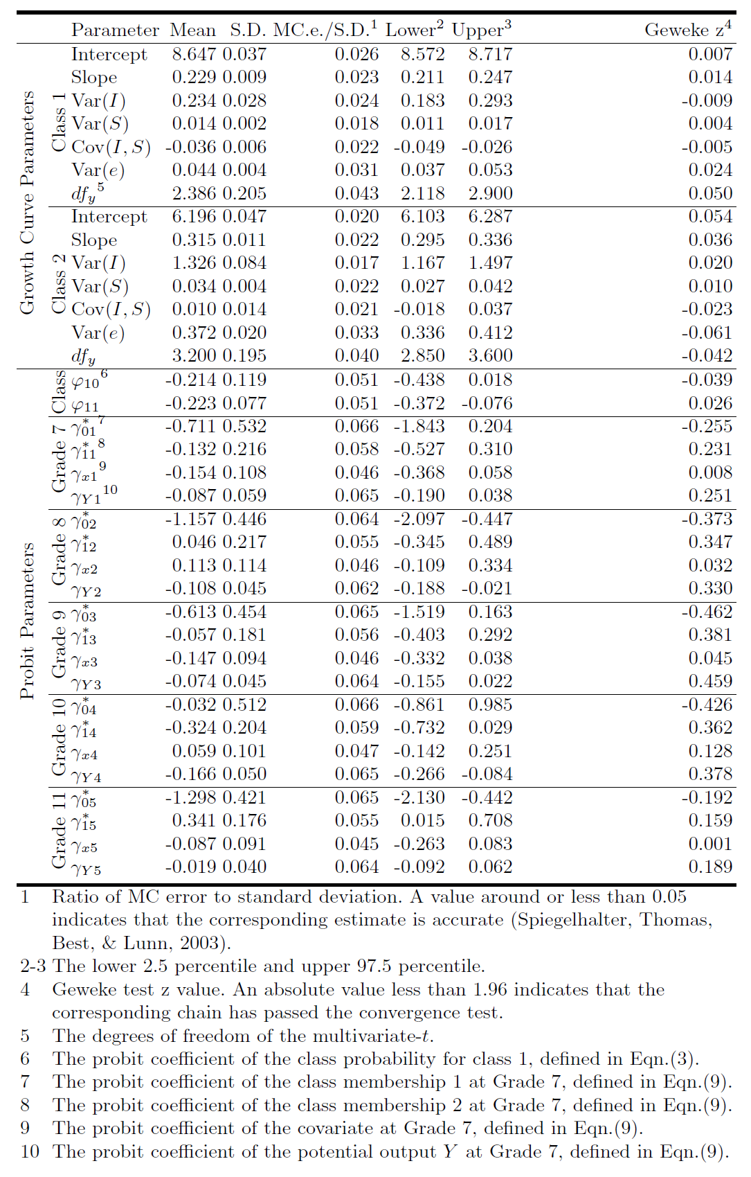
As suggested by Dhat.CAIC, Dhat.ssBIC, Dhat.BIC, and Dhat.AIC, without further substantive information, the TN-CXY model appears to be a good candidate for the best-fitting model. Table 10 provides the results of the TN-CXY REGMM model. It can be seen that (1) class 1 has a higher average initial level but a smaller average slope; (2) class 2 has larger variations for initial levels and slope; (3) the residual variance of class 2 is much larger than that of class 1; (4) in class 1 the initial level and the slope are significantly negatively correlated at the confidence level of 95%; (5) the missingness is not related to gender because none of the coefficients of gender are significant at the $\alpha $ level of $0.05$; (6) at grade 11, adolescents in class 2 are more likely to miss tests than those in class 1 because the probit coefficient of class membership for grade 11 is significantly positive; and (7) at grades 8 and 10, students with higher potential scores are more likely to miss tests than the students having lower scores because the probit coefficients of the potential outcomes $y$ at the two grades are significantly negative.
Based on the results from the five simulation studies, one can conclude that (1) almost all of the model selection indices, except for the rough DIC (RDIC), can correctly choose the true model with high certainty; (2) if the number of classes is correctly identified, then the Dbar-based indices perform better than the Dhat-based indices; if candidate models have different numbers of classes, then the Dhat-based indices might be used to select the best fit model; (3) across 5 studies, CAIC and BIC provide higher probabilities than those ssBIC, AIC, or DIC does. The results will help inform the selection of growth models by researchers seeking to provide people with accurate estimates of growth across a variety of possible contexts. The real data analysis demonstrated the application of the indices to typical longitudinal growth studies such as educational, psychological, and social research.
This study can be extended in many ways. For example, different versions of the likelihood function or more model selection indices can be studied and compared by using more practical statistical models. (1) As we stated in the section of Introduction, there are at least three challenges in proposing new selection indices. The third challenge is about the likelihood function $l(y|\hat {\theta })$. When latent variables involved, the likelihood can be an observed-data likelihood, a complete-data likelihood, or a conditional likelihood (Celeux et al., 2006). In this study, we use a conditional joint loglikelihood, but in the future, the other versions of likelihood functions can be investigated. (2) Another future research of this study is to propose other model selection indices, such as Bayes factors. (3) This study focuses on latent growth models only. In the future, the performance of these selection indices can be studied by using other statistical models, such as survival models.
The study was supported by a grant from the Institute of Education Sciences (R305D210023).
Akaike, H. (1974). A new look at the statistical model identification. IEEE Transactions on Automatic Control, 1919 (6), 716-723. doi: https://doi.org/10.1007/978-1-4612-1694-0_16
Anderson, T. W., & Bahadur, R. R. (1962). Classification into two multivariate normal distributions with different covariance matrices. The Annals of Mathematical Statistics, 33, 420-431. doi: https://doi.org/10.1214/aoms/1177704568
Bartholomew, D. J., & Knott, M. (1999). Latent variable models and factor analysis: Kendall’s library of statistics (2nd ed., Vol. 7). New York, NY: Edward Arnold.
Bozdogan, H. (1987). Model selection and Akaike’s Information Criterion (AIC): The general theory and its analytical extensions. Psychometrika, 52, 345-370. doi: https://doi.org/10.1007/bf02294361
Bureau of Labor Statistics, U.S. Department of Labor. (1997). National longitudinal survey of youth 1997 cohort, 1997-2003 (rounds 1-7). [computer file]. Produced by the National Opinion Research Center, the University of Chicago and distributed by the Center for Human Resource Research, The Ohio State University. Columbus, OH: 2005. Retrieved from http://www.bls.gov/nls/nlsy97.htm
Casella, G., & George, E. I. (1992). Explaining the Gibbs sampler. The American Statistician, 46(3), 167-174. doi: https://doi.org/10.2307/2685208
Celeux, G., Forbes, F., Robert, C., & Titterington, D. (2006). Deviance information criteria for missing data models. Bayesian Analysis, 4, 651-674. doi: https://doi.org/10.1214/06-ba122
Dunson, D. B. (2000). Bayesian latent variable models for clustered mixed outcomes. Journal of the Royal Statistical Society, B, 62, 355-366. doi: https://doi.org/10.1111/1467-9868.00236
Geweke, J. (1992). Evaluating the accuracy of sampling-based approaches to calculating posterior moments. In J. M. Bernado, J. O. Berger, A. P. Dawid, & A. F. M. Smith (Eds.), Bayesian statistics 4 (p. 169-193). Oxford, UK: Clarendon Press.
Glynn, R. J., Laird, N. M., & Rubin, D. B. (1986). Drawing inferences from self-selected samples. In H. Wainer (Ed.), (p. 115-142). New York: Springer Verlag.
Little, R. J. A. (1993). Pattern-mixture models for multivariate incomplete data. Journal of the American Statistical Association, 88, 125-134. doi: https://doi.org/10.2307/2290705
Little, R. J. A. (1995). Modelling the drop-out mechanism in repeated-measures studies. Journal of the American Statistical Association, 90, 1112-1121. doi: https://doi.org/10.1080/01621459.1995.10476615
Little, R. J. A., & Rubin, D. B. (2002). Statistical analysis with missing data (2nd ed.). New York, N.Y.: Wiley-Interscience. doi: https://doi.org/10.1002/9781119013563
Lu, Z., & Zhang, Z. (2014). Robust growth mixture models with non-ignorable missingness data: Models, estimation, selection, and application. manuscript submitted for publication. Computational Statistics and Data Analysis, 71, 220–240. doi: https://doi.org/10.1016/j.csda.2013.07.036
Lu, Z., & Zhang, Z. (2021). Bayesian approach to non-ignorable missingness in latent growth models. Journal of Behavioral Data Science, 1(2), 1–30. doi: https://doi.org/10.35566/jbds/v1n2/p1
Lu, Z., Zhang, Z., & Cohen, A. (2013). New developments in quantitative psychology. In R. E. Millsap, L. A. van der Ark, D. M. Bolt, & C. M. Woods (Eds.), (Vol. 66, p. 275-304). Springer New York.
Lu, Z., Zhang, Z., & Lubke, G. (2011). Bayesian inference for growth mixture models with latent-class-dependent missing data. Multivariate Behavioral Research, 46, 567-597. doi: https://doi.org/10.1080/00273171.2011.589261
Maronna, R. A., Martin, R. D., & Yohai, V. J. (2006). Robust statistics: Theory and methods. John Wiley & Sons, Inc. doi: https://doi.org/10.1002/0470010940
McLachlan, G. J., & Peel, D. (2000). Finite mixture models. New York, NY: John Wiley & Sons. doi: https://doi.org/10.1002/0471721182
Muthén, B., & Shedden, K. (1999). Finite mixture modeling with mixture outcomes using the EM algorithm. Biometrics, 55(2), 463-469. doi: https://doi.org/10.1111/j.0006-341x.1999.00463.x
Oldmeadow, C., & Keith, J. M. (2011). Model selection in Bayesian segmentation of multiple DNA alignments. Bioinformatics, 27, 604-610. doi: https://doi.org/10.1093/bioinformatics/btq716
Schwarz, G. E. (1978). Estimating the dimension of a model. Annals of Statistics, 6 (2), 461-464. doi: https://doi.org/10.1214/aos/1176344136
Sclove, L. S. (1987). Application of mode-selection criteria to some problems in multivariate analysis. Psychometrics, 52, 333-343. doi: https://doi.org/10.1007/bf02294360
Spiegelhalter, D. J., Best, N. G., Carlin, B. P., & Linde, A. v. d. (2002). Bayesian measures of model complexity and fit. Journal of the Royal Statistical Society: Series B (Statistical Methodology), 64(4), 583-639. doi: https://doi.org/10.1111/1467-9868.00353
Spiegelhalter, D. J., Thomas, A., Best, N., & Lunn, D. (2003). WinBUGS manual Version 1.4.
(MRC Biostatistics Unit, Institute of Public Health, Robinson Way, Cambridge CB2 2SR, UK, http://www.mrc-bsu.cam.ac.uk/bugs)
Yuan, K.-H., & Lu, Z. (2008). SEM with missing data and unknown population using two-stage ML: theory and its application. Multivariate Behavioral Research, 43, 621-652. doi: https://doi.org/10.1080/00273170802490699
Zhang, Z., Lai, K., Lu, Z., & Tong, X. (2013). Bayesian inference and application of robust growth curve models using student’s t distribution. Structural Equation Modeling, 20(1), 47-78. doi: https://doi.org/10.1080/10705511.2013.742382


![----- ∑S ∑N ∑T
ED |y[D(θ)] ≈ D(θ) = --2 l(is)t (θ|y,m )
S s=1 i=1 t=1
∑S ∑N ∑T [ ]
= - -2 (1 - m (is)t )l(ist) (y)+ l(sit)(m) , (10)
S s=1 i=1 t=1](v2n1p29x.svg)
 τimtit, (11)](v2n1p210x.svg)
![N T
D (E [θ]) ≈ D(ˆθ) = - 2∑ ∑ [(1- m )l(y|ˆθ)+ l(m |θˆ)], (12)
θ|y i=1t=1 it it it](v2n1p211x.svg)
![----- 2 S∑ N∑ K∑ ∑T [ ]
ED|y[D (θ)] ≈ D (θ) = -- z(sik) (1- mit)l(isk)t(y)+ l(sik)t(m ) ,(13)
S s=1 i=1 k=1 t=1](v2n1p212x.svg)
![N K T [ ]
D(E [θ]) ≈ D (ˆθ) = - 2∑ ∑ zˆ ∑ (1- m )l (y|ˆθ)+ l (m |ˆθ) , (14)
θ|y i=1k=1 ikt=1 it ikt ikt](v2n1p213x.svg)