Keywords: Robust methods · Growth curve modeling · Conditional medians · Laplace distribution
Longitudinal data track the same subjects across different time points. In contrast to cross-sectional data, longitudinal data allow for measuring the within-subject change over time, capturing the duration of events, and recording the timing of various events. Growth curve modeling is one of the most frequently used analytical techniques for longitudinal data analysis (e.g., McArdle & Nesselroade, 2014), due to its abilities to examine within-subject change over time, and to investigate into differences of the change patterns among individuals.
In growth curve modeling, estimation methods that are based on the normality assumption in data distribution are widely accepted, and have been incorporated in many statistical software packages. When data all come from a normal population, those methods are able to provide consistent and efficient parameter estimators. However, practical data are often contaminated with outlying observations in social and behavioral sciences, so that the normality assumption is violated in real data analysis. For example, Micceri (1989) investigated 440 large-scale data sets in psychology and found that almost all of them were significantly nonnormal. When the normality assumption does not hold, traditional growth curve modeling which focuses on conditional means of the outcome variables may lead to inefficient and even biased model estimation (e.g., Yuan & Bentler, 2001).
To disentangle the influence of data contamination, the cause of the contamination needs to be understood. Reflected in growth curve modeling, data contamination may be caused by extreme scores in either random effects or within-subject measurement errors. The former is referred to as leverage observations and the latter is called outliers (Tong & Zhang, 2017). It is necessary to distinguish these two types of outlying observations since their influences on the estimation of growth curve models (GCMs) are different. Although techniques to detect leverage observations and outliers have been developed (e.g., Tong & Zhang, 2017), it has been shown that outlying observation detection in longitudinal data is a challenging problem whose sensitivity and specificity are difficult to guarantee. Even if the leverage observations and outliers are correctly identified, simply deleting them could result in decreased statistical efficiency (Lange, Little, & Taylor, 1989).
To address the issue of data contamination, various robust estimation methods have been proposed to produce reliable analysis in the presence of data nonnormality. Some of them rely on making distributional assumptions that are more reasonable to the dataset, such as using Student’s t distributions or mixture of normal distributions (Lu & Zhang, 2014; Reich, Bondell, & J., 2010; Tong & Zhang, 2012). However, those methods are sensitive to the choice of the assumed distribution, which is difficult to specifiy a priori and verify afterwards, especially for small sized data. Another genre of robust methods assign weights to observations according to their distances from the center of the majority of data so that extreme cases are downweighted (e.g., Pendergast & Broffitt, 1985; Singer & Sen, 1986; Yuan & Bentler, 1998a; Zhong & Yuan, 2010). Those weighting methods may have limitations under certain conditions, e.g., in general, they do not take the leverage observations into consideration (Zhong & Yuan, 2011).
Median-based regression and its generalization, quantile regression (Koenker, 2004), have emerged as another genre of robust methods. Such methods are distribution free, and have been extended to many topics such as penalized regression and time series models. Although the median-based methods are still not widely applied to longitudinal research (Geraci, 2014), they are getting more and more attention (e.g., Cho, Hong, & Kim, 2016; Galvao & Poirier, 2019; Huang, 2016; Smith, Fuentes, Gordon-Larsen, & Reich, 2015; Zhang, Huang, Wang, Chen, & Langland-Orban, 2019). Recently a robust growth curve modeling approach using conditional medians was proposed (Tong, Zhang, & Zhou, 2021). Although this robust approach outperformed traditional conditional mean-based growth curve modeling in the presence of outliers, it still yielded biased parameter estimates when leverage observations exist.
It is crucial to have a robust estimator for growth curve models when data are contaminated with both outliers and leverage observations in longitudinal studies. To obtain such an estimator, we develop a DOuble MEdian-based structure (DOME) to mitigate potential distortion in both distributions of random effects and of within-subject measurement errors in growth curve modeling. When random effects and measurement errors are symmetrically distributed, the estimates based on the developed method will be very close to the ones obtained by traditional growth curve modeling estimation method. It is expected that DOME growth curve modeling is more robust against nonnormal data than traditional conditional mean-based method, and also outperforms the median-based growth curve modeling in Tong et al. (2021). Bayesian methods are used for DOME GCM estimation because they can conveniently infer parameters that do not have symmetric distributions (e.g., variance parameters), incorporate prior information to make parameter estimates more efficient, naturally accommodate missing data without requiring new techniques, and are powerful to deal with complex model structures.
In sum, the purpose of this work is to develop a robust Bayesian growth curve modeling approach that is effective to analyze longitudinal data that are contaminated with both outliers and leverage observations in general. In the following sections, the idea of the proposed robust approach, DOME GCM, will be introduced, Monte Carlo simulation studies are conducted to evaluate the numerical performance of the developed method and compare its performance with those of traditional growth curve modeling and the median-based method developed by Tong et al. (2021), and an empirical example is provided to illustrate the application of DOME GCM to study the change of memory scores using a real dataset from the Virginia Cognitive Aging Project (Salthouse, 2014, 2018). We conclude this article with discussions and suggestions on future research directions.
In longitudinal studies, the same subjects are measured repeatedly over time. Suppose that a longitudinal study is conducted on a cohort of individuals, indexed by $i=1,...,N$. Let $\boldsymbol {y}_{i}=(y_{i1},...,y_{iT_i})^\intercal $ be a $T_i \times 1$ vector, where $y_{it}$ is the observation on individual $i$ at time $t$ for $t=1,...,T_i$ with $T_i$ being the maximum follow-up time for this individual. A typical form of the unconditional GCMs can be formulated as
| (1) |
where $\boldsymbol {X}_i$ is a $T_i\times q$ factor loading matrix recording the time of measurements. It can be different across individuals when they are not measured at a common set of time. The vector $\boldsymbol {b}_{i}$ is a $q\times 1$ vector of random effects, and $\boldsymbol {\epsilon }_{i}$ is a vector of within-subject measurement errors. The vector of random effects $\boldsymbol {b}_{i}$ varies across individuals, and $\boldsymbol {\beta }$ represents the fixed effects for the population. The residual vector $\boldsymbol {u}_{i}$ represents the random component of $\boldsymbol {b}_{i}$. Without loss of generality, we assume the number of measurement occasions to be the same for all individuals, i.e., $T_i \equiv T$.
Traditional GCMs typically assume that both $\boldsymbol {\epsilon }_{i}$ and $\boldsymbol {u}_{i}$ follow multivariate normal (MN) distributions,
 |
where the subscripts of MN distributions imply the dimensionalities of the random vectors. The covariance matrix $\boldsymbol {\Phi }$ is usually assumed to be diagonal $\boldsymbol {\Phi }=\sigma _{\epsilon }^{2}\boldsymbol {I}$, indicating that measurement errors have equal variance and are independent across different time points.
Traditional GCMs focus on modeling the conditional means of the outcome variables, $E(\boldsymbol {y}_{i}|\boldsymbol {b}_i)=\boldsymbol {X}_i\boldsymbol {b}_{i}$, and estimating the common growth parameters, $E(\boldsymbol {b}_{i})=\boldsymbol {\beta }$.
However, it is well known that mean is sensitive to outlying observations. Tong et al. (2021) proposed a median-based GCM where the conditional medians of the outcome variables $Q_{0.5}(\boldsymbol {y}_i|\boldsymbol {b}_i)$, are examined instead of the conditional means $E(\boldsymbol {y}_{i}|\boldsymbol {b}_i)$. Their numerical results showed that this approach is only robust against outliers, but not against leverage observations. This is as expected because an outlier is caused by an extreme score in $\boldsymbol {\epsilon }_i$ and a leverage observation is caused by an extreme score in $\boldsymbol {u}_i$. The robust approach in Tong et al. (2021) only models the conditional medians of the outcome variables at the level-one model. Although it seems to be a natural extension to model conditional medians of the level-two model as well to address the influence of leverage observations, the extension is not straightforward because within-subject measurement errors $\boldsymbol {\epsilon }_{i}$ were assumed to be independent across different time points and can be modeled as univariate random variables, whereas $\boldsymbol {u}_i$ has to be specified as a multivariate variable with dependent components.
In this paper, we tackle the complicated multivariate problem and propose a robust method by adopting two median structures as alternatives, $Q_{0.5}(\boldsymbol {y}_i|\boldsymbol {b}_i)$ replacing $E(\boldsymbol {y}_{i}|\boldsymbol {b}_i)$ and $Q_{0.5}(\boldsymbol {b}_i)$ replacing $E(\boldsymbol {b}_{i})$. We call this new model a double medians growth curve model (DOME GCM).
As discussed previously, outlying observations in longitudinal data can be either outliers as a result of extreme measurement errors, or leverage observations due to extreme scores in random effects (Tong & Zhang, 2017). The proposed DOME GCM aims to handle the presence of data nonnormality due to both types of outlying observations.
DOME growth curve modeling is an extension of traditional mean-based method,
| (2) |
where medians for vector are taken entry-wise. In this multilevel modeling framework, at the first level, the relationship between $\boldsymbol {X}_i$ and the outcome variable $\boldsymbol {y}_i$ is based on the conditional median function $Q_{0.5}(\boldsymbol {\epsilon }_i|\boldsymbol {u}_i) = \boldsymbol {0}$. At the second level, random effect $\boldsymbol {b}_i$ varies around the median $\boldsymbol {\beta }$, the fixed effects for the population. The random residuals $\boldsymbol {u}_i = [u_{i1}, u_{i2}, \dots , u_{iq}]^\intercal $ are the random components of $\boldsymbol {b}_i$. Since no distributional assumption is imposed on $\boldsymbol {\epsilon }_i$ or $\boldsymbol {u}_i$, the proposed DOME growth curve model is distribution-free.
The multilevel structure in Equation (2) can be expressed compactly as
| (3) |
where $Q_{0.5}({\epsilon }_{it}|\boldsymbol {u}_i) = 0$ and $Q_{0.5}(\boldsymbol {u}_{i}) = 0$. Here $\boldsymbol {x}_{it}$ is the transpose of the $t$th row of $\boldsymbol {X}_i$. The population regression coefficient $\boldsymbol {\beta }$ is the main parameter of interest in the DOME GCM model.
Recall that in traditional regression based on conditional means, we minimize the sum of squared residuals to estimate model parameters. Similarly, in a median-based regression,

estimation is carried out by minimizing the sum of absolute residuals,
| (4) |
However, this minimization involves the sum of absolute values, which is not differentiable at zero, meaning that explicit solutions to the minimization problem are unavailable. Moreover, when more than one median constraints are introduced, as in the case of the DOME GCM model in Equations (2), defining an objective function similar to Equation (4) becomes difficult, for the reason that the objective function should be marginalized and involves integration. The computational challenge can be overcome by introducing Laplace distributions to make a connection between the estimation of DOME GCM in Equations (2) and the maximum likelihood principle (Geraci, 2014).
The Laplace distribution has a relationship with the $l_{1}$-norm loss function described in Koenker and Bassett (1978). This relationship is best demonstrated by the probability density function for a unidimensional Laplace distribution $X \sim Laplace(\mu ,\sigma )$,

where $\mu \in R$ is the location parameter and $\sigma \in R_{+}$ is the scale parameter. The mean and variance of the distribution are given by
 |
respectively. Laplace distribution is also known as the standard double exponential distribution.
The univariate Laplace distribution can be extended to the multivariate Laplace distribution (Kozubowski & Podgorski, 2000). The marginal distributions of a multivariate Laplace distribution variable are unidimensional Laplace distributions. A multivariate Laplace distribution is parameterized by location $\boldsymbol {\mu }$ and covariance matrix $\boldsymbol {\Sigma }$, denoted as $\boldsymbol {Y} \sim Laplace(\boldsymbol {\mu }, \boldsymbol {\Sigma })$. For a $n$-dimensional Laplace distribution, if $\boldsymbol {\mu } = 0$, the probability density function of the multivariate Laplace distribution is given by

where $v = \frac {2-n}{2}$ and $K_v$ is the modified Bessel function of the second kind.
We employ Laplace distributions to convert the problem of estimating DOME GCM into a problem of obtaining the maximum likelihood estimator (MLE) for a transformed model. For the purpose of demonstration, we focus on a linear GCM in this paper, so that the random effect is two-dimensional
![[L]
bi = Si ,
i](v2n2p19x.svg)
where $L_i$ is the initial level and $S_i$ is the rate of change over time for the $i$th individual, respectively. The transformed model for the DOME GCM in Equations (2) is
| (5) |
Note that the median structures are applied for the measurement errors using a univariate Laplace distribution, and for the random effects using a bivariate Laplace distribution. Since the median of a Laplace distribution is the location parameter $\mu $, it can be verified that
 |
so that parameter estimation of DOME GCM in Equations (2) can be obtained by estimating the transformed model in Equations (5), for which the likelihood function for $T$ observations across $N$ subjects is
| (6) |
where $p(\boldsymbol {y}_i|\boldsymbol {b}_i, \boldsymbol {\beta }, \sigma _\epsilon )$ is the conditional probability density function of $\boldsymbol {y}_i$ and $p(\boldsymbol {b}_i|\boldsymbol {\beta }, \Sigma )$ is the probability density function for multivariate Laplace distribution.
The solution of the maximum likelihood problem is difficult to derive analytically, or numerically under the frequentist framework, as $\boldsymbol {b}_i$’s need to be integrated out. Alternatively, the estimation can be carried out naturally under the Bayesian framework, as Bayesian methods with data augmentation techniques are flexible and computationally more powerful in such settings. Monte Carlo Markov Chain (MCMC) algorithms can be applied here, using empirical integration to approximate the exact integration. The basic idea of Bayesian methods is to obtain the posterior distributions of model parameters based on the likelihood function and the priors. Since the Laplace distribution can be constructed using a normal distribution and an exponential distribution, the data augmentation technique is used here to simplify the procedure to obtain posterior distributions. Specifically, to simulate a Laplace distribution with location $\boldsymbol {\mu }$ and covariance matrix $\boldsymbol {\Sigma }$, we can generate, independently, two augmented variables $W \sim exp(1)$ and $\boldsymbol {X} \sim N(0, \boldsymbol {\Sigma })$. As a result, the variable

follows the $Laplace(\boldsymbol {\mu }, \boldsymbol {\Sigma })$ distribution. The augmented representation provides an efficient method to draw MCMC from the posterior distribution. Particularly, if conjugate priors are used, we can derive conditional posterior distribution for the model parameters. Gibbs sampling then can be utilized, where samples of parameters are drawn iteratively from the conditional posterior distribution. This way we obtain the empirical marginal distribution of model parameters, with which model estimation and statistical inference can be performed. Noninformative conjugate priors are used in our study because of their advantage in easy Gibbs sampling derivation. Other priors, especially informative priors when previous information is available, can also be used and may be more advantageous, on potentially reducing convergence issue or decreasing computation time (e.g., Depaoli, Liu, & Marvin, 2021).
In this section, a simulation study is conducted to evaluate the numerical performance of the robust Bayesian DOME growth curve modeling in analyzing contaminated data with outliers and/or leverage observations, which correspond to extreme scores in measurement errors and random effects, respectively. Comparisons are drawn among the developed DOME GCM, traditional growth curve modeling based on conditional means, as well as the robust Bayesian method in Tong et al. (2021) where the median structure is only applied in the first level of GCM, referred to as the median-based method hereafter.
To directly compare with the study in Tong et al. (2021), we follow their simulation design and focus on the linear GCM as discussed in the previous section. The number of measurement occasions is set at 5, the population parameter values for the fixed effects are set as $\boldsymbol {\beta } = (\beta _L, \beta _S)^\intercal = (6.2, 1.5)^\intercal $, the variance of latent intercept $\sigma _L^2 = 0.5$, the variance of latent slope $\sigma _S^2 = 0.1$, the covariance between intercept and slope is 0, and the measurement error variance $\sigma _\epsilon ^2=0.1$.
In the simulation, we vary the sample size ($N = 200, 500$), the percentage of outlying observations ($10\%, 25\%$), and the types of outlying observations (outliers and leverage observations). Given a specific sample size and the percentage of outlying observations $r\%$, we first generate normally distributed measurement errors $\boldsymbol {\epsilon }_i \sim MN_5(0, \sigma _\epsilon ^2\boldsymbol {I})$ and random effects $\boldsymbol {u_i} \sim MN_2(0, \Phi )$. Then $r\%$ of subjects are randomly selected to be contaminated by outlying observations in three scenarios; all selected subjects are contaminated by outliers, all selected subjects are contaminated by leverage observations, and the selected subjects are randomly contaminated with outliers or leverage observations with equal probabilities.
To generate outliers, we randomly select 2 out of the 5 observations for one subject, and replace them by data generated from $N(0, 0.1)$. To generate leverage observations, the random slopes of the contaminated subjects are set to follow the distribution $N(-3, 0.1)$, instead of $N(1.5, 0.1)$ for the population.
For each data condition, a total of 500 datasets are generated. Each dataset is analyzed using the three methods. Traditional growth curve modeling with normality assumptions is conducted under the structural equation modeling framework, using the ”lavaan” package in R (Rosseel, 2012). The median-based method and the proposed DOME growth curve modeling are implemented with the ”rstan” package (Stan Development Team, 2019). The Markov chain length is set to be 15,000, and the burn-in period is 7,500. A set of commonly used priors are specified for model parameters. A multivariate normal distribution prior is assumed for $\boldsymbol {\beta }$. The measurement error variance $\sigma ^2_\epsilon $ is given an inverse gamma prior, and inverse Wishart distribution is assumed for the covariance of random effect $\boldsymbol {\Sigma }$. More details can be found in the R code for implementation in the appendix.
We obtain parameter estimation based on the three methods. Estimation bias, empirical standard error (ESE), average standard error (ASE), and mean squared error (MSE) for each parameter are calculated and used to evaluate the numerical performances of those methods. Let $\theta $ denote a parameter and also its population value, and let $\hat {\theta }_k$ and $SE_k$ denote its estimate and the corresponding estimated standard error in the $k$th replication. Then the parameter estimate of $\theta $, $\hat {\theta }$, is calculated as the average of parameter estimates of 500 simulation replications

The bias of $\hat {\theta }$ is $bias(\hat {\theta }) = \hat {\theta } - \theta $. The empirical standard error is defined by

The average standard error is

When standard errors are estimated accurately in model estimation by the developed method, ASE should be very close to ESE. The mean squared error is calculated by $MSE(\hat {\theta }) = bias^2 + ESE^2$. A smaller MSE indicates a more accurate and precise estimator.
When Bayesian methods are applied, Geweke tests (Geweke, 1992) are used to assess the convergence of Markov chains for all simulation replications. After the burn-in period, if sample parameter values are drawn from the stationary distribution of the chain, the means of the first and last parts of the Markov chain (by convention the first 10% and the last 50 %) should be equal, and the Geweke statistic asymptotically follows a standard normal distribution. We report the convergence percentage of the 500 replications by Geweke test, and the summarized model estimation results are based only on converged replications. In practice, if the MCMC procedure does not converge, we may adopt longer Markov chains, or choose different starting values or prior distributions to yield convergent Markov chains.
The model estimation time, in the number of seconds, is reported for the two Bayesian methods. The median estimation time (MET) is the median of the estimation time for the converged replications.
When there are no outlying observations, traditional mean-based growth curve modeling and the two robust median based growth curve modeling approaches perform equally well.
Tables 1 - 2 summarize the parameter estimation results for the overall latent slopes ($\beta _S$) and the variance of latent slopes ($\sigma _S^2$), respectively, with the sample size $N = 200$. The overall latent slope and variance of latent slopes are chosen as the parameters of interest, based on the presumption that substantive researchers using growth curve models are most often interested in assessing changes over time. Results for other model parameters and for $N=500$ have similar patterns and are given in the supplementary file: https://github.com/CynthiaXinTong/DOME. When the sample size is 200, Geweke tests suggest that at least $91\%$ replications converged. We summarize the estimation results based on those converged Markov chains.
| Type | r% | Method | Est | Bias | MSE | ASE | ESE | CR | MET |
Outlier |
10% | Mean | 1.33 | -0.17 | 29.5 | 4.62 | 3.07 | NA | |
| Median | 1.48 | -0.02 | 1.21 | 2.50 | 2.42 | 94.2 | 1149 | ||
| DOME | 1.48 | -0.02 | 1.28 | 2.77 | 2.65 | 96 | 1551 | ||
25% | Mean | 1.06 | -0.44 | 194.6 | 6.30 | 3.62 | NA | ||
| Median | 1.44 | -0.06 | 4.73 | 3.19 | 2.78 | 94.4 | 740 | ||
| DOME | 1.43 | -0.07 | 5.17 | 3.35 | 3.05 | 95.8 | 1362 | ||
Leverage |
10% | Mean | 1.05 | -0.45 | 202 | 9.82 | 2.26 | NA | |
| Median | 1.05 | -0.45 | 204 | 8.39 | 2.64 | 94.6 | 2583 | ||
| DOME | 1.44 | -0.06 | 5.32 | 4.21 | 3.17 | 93.4 | 2412 | ||
25% | Mean | 0.37 | -1.13 | 1269 | 14.0 | 2.35 | NA | ||
| Median | 0.37 | -1.13 | 1270 | 10.8 | 3.02 | 95.6 | 2963 | ||
| DOME | 1.29 | -0.21 | 47.1 | 7.35 | 4.09 | 94.6 | 2674 | ||
50-50 Mix |
10% | Mean | 1.19 | -0.31 | 98.0 | 7.80 | 4.27 | NA | |
| Median | 1.21 | -0.29 | 86.2 | 7.05 | 5.40 | 95.0 | 2200 | ||
| DOME | 1.45 | -0.05 | 3.00 | 3.65 | 2.92 | 97.0 | 2072 | ||
25% | Mean | 0.72 | -0.78 | 611 | 11.1 | 5.67 | NA | ||
| Median | 0.77 | -0.73 | 545 | 9.69 | 7.56 | 94.6 | 1819 | ||
| DOME | 1.36 | -0.14 | 21.3 | 2.31 | 3.37 | 93.6 | 1936 | ||
Note. Est = Estimate; CR = convergence rate; MET = median estimation time in seconds; 50-50 Mix: data contain outliers and leverage observations with equal probabilities. MSE was multiplied by 1000 and ASE and ESE were multiplied by 100.
| Type | r% | Method | Est | Bias | MSE | ASE | ESE | CR | MET |
Outlier |
10% | Mean | 0.25 | 0.15 | 26.36 | 4.71 | 5.60 | NA | |
| Median | 0.07 | -0.03 | 1.02 | 1.31 | 1.26 | 93.8 | 982 | ||
| DOME | 0.16 | 0.06 | 8.98 | 3.21 | 6.92 | 95.4 | 1263 | ||
25% | Mean | 0.39 | 0.29 | 88.57 | 8.74 | 7.04 | NA | ||
| Median | 0.06 | -0.04 | 1.66 | 1.53 | 1.07 | 94.8 | 619.28 | ||
| DOME | 0.13 | 0.03 | 1.51 | 4.68 | 11.97 | 93.6 | 1154 | ||
Leverage |
10% | Mean | 1.92 | 1.82 | 3326 | 19.32 | 6.33 | NA | |
| Median | 1.93 | 1.83 | 3350 | 19.27 | 6.68 | 94.6 | 2253 | ||
| DOME | 0.96 | 0.86 | 750 | 13.78 | 4.43 | 94.0 | 2087 | ||
25% | Mean | 3.90 | 3.80 | 14440 | 39.08 | 9.90 | NA | ||
| Median | 3.91 | 3.81 | 14503 | 38.74 | 11.46 | 94.8 | 2792 | ||
| DOME | 3.64 | 3.55 | 12592 | 51.48 | 13.78 | 96.0 | 2279 | ||
50-50 Mix |
10% | Mean | 1.13 | 1.13 | 1098.89 | 12.30 | 20.06 | NA | |
| Median | 0.11 | 0.01 | 10.32 | 34.41 | 10.13 | 91.0 | 2196 | ||
| DOME | 0.18 | 0.08 | 41.08 | 57.74 | 18.41 | 93.0 | 2071 | ||
25% | Mean | 2.26 | 2.16 | 4737.37 | 216.05 | 26.35 | NA | ||
| Median | 0.11 | 0.01 | 15.65 | 1.05 | 12.47 | 92.6 | 1819 | ||
| DOME | 0.51 | 0.41 | 277.74 | 41.60 | 32.35 | 94.4 | 1968 | ||
Note. Same as Table 1 | |||||||||
When data contain outliers but no leverage observation exists, our proposed DOME growth curve modeling yields parameter estimates that are very similar to those from the conditional median-based method, and are less biased than those from traditional mean-based method. Both MSEs and standard errors from the two robust Bayesian methods are smaller than those from the traditional mean growth curve model, indicating that the proposed method is on par with conditional median-based method, and is more efficient than traditional growth curve modeling. This pattern is more salient when the proportion of outliers increases. Note that for DOME growth curve modeling, standard errors of $\sigma _S^2$ are underestimated, as ASEs are smaller than ESEs. This may be due to the autocorrelations of the Markov chains, and could potentially be overcome by thinning the Markov chains. In sum, the DOME growth curve modeling is more robust against outliers than traditional mean-based growth curve modeling. It provides less biased and more efficient parameter estimators. The conditional median-based method performs similarly as the DOME growth curve modeling on handling outliers.
When data contain leverage observations but no outliers, the advantage of the DOME GCM becomes apparent. In this situation, both traditional mean-based method and the conditional median-based growth curve modeling break down, yielding similar parameter estimates. But the estimates by DOME GCM are much less biased. For example, as shown in Table 1, when the proportion of leverage observations is $10\%$, the estimation bias for $\beta _S$ is -0.45 for both traditional mean-based method and the robust median-based method. DOME growth curve modeling can substantially reduce the bias to -0.06. This is mainly because the conditional median-based method only applies medians in the first level of the growth curve model, whereas leverage observations are extreme values in the second level. Note that standard errors in the DOME growth curve modeling is overestimated as ASEs are larger than ESEs. However, ASEs estimated by the DOME GCM method are still closer to their corresponding ESEs than the ASEs estimated by the other two methods.
When data contain both outliers and leverage observations, DOME growth curve modeling still performs much better than the mean-based method and the median-based method in terms of estimation bias and efficiency. In general, when data are suspected to be contaminated, DOME GCM should be a preferred method than the traditional GCM and conditional median-based GCM.
It is probably counter-intuitive that the MET is shorter when the proportion of outliers is higher. This is consistent with the findings in Tong et al. (2021). In MCMC sampling, Markov chains typically have trouble exploring high curvature regions. A small proportion of outliers (e.g., 10%) creates a steep and high curvature region for the chain to enter, and thus the computing time tends to be longer. As the proportion increases, the curvature becomes smoother and the MCMC procedure is faster.
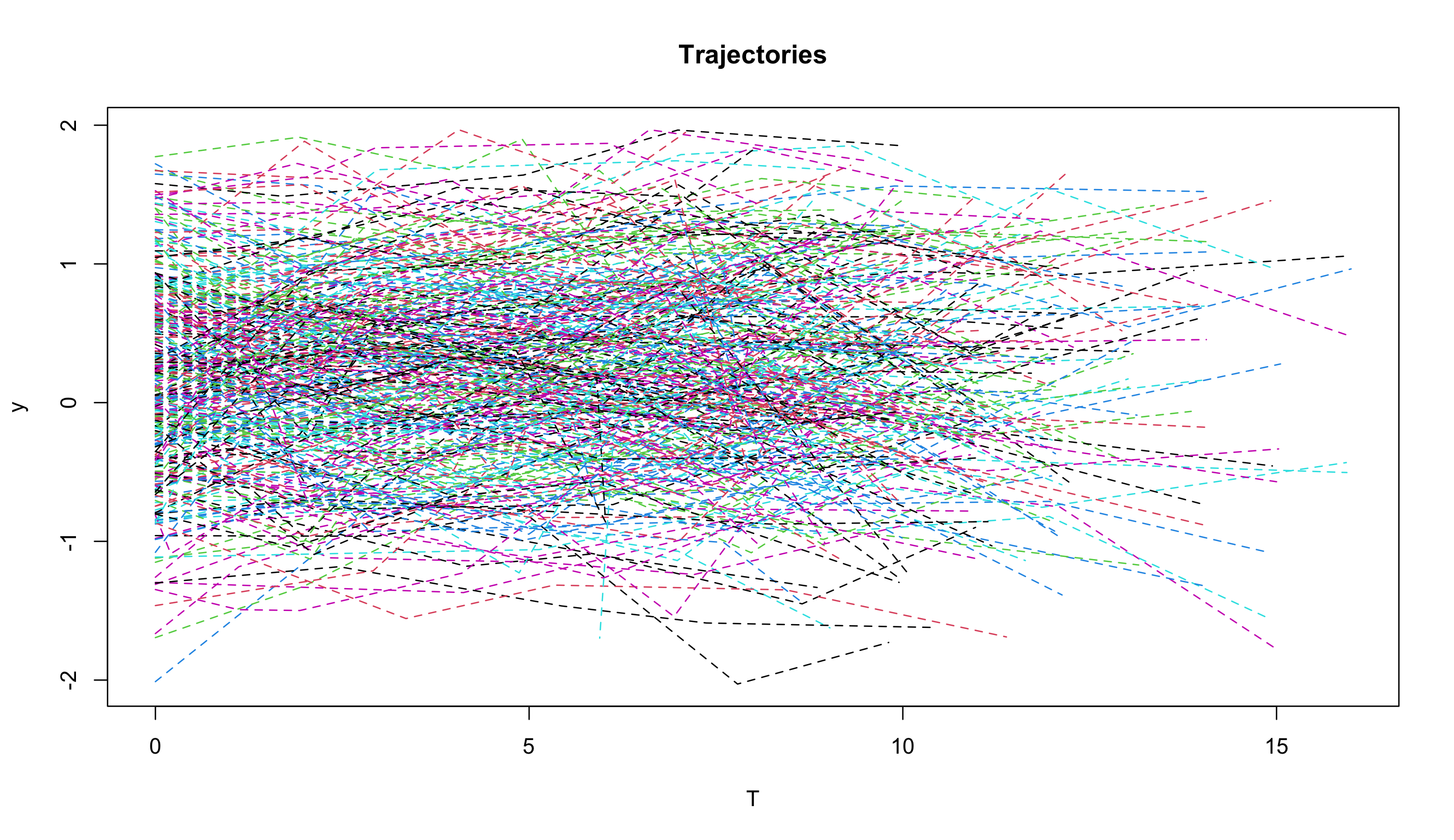
To demonstrate its application, we apply the proposed DOME GCM to a subset of data from the Virginia Cognitive Aging Project (VCAP; Salthouse 2014, 2018). VCAP, starting in 2001, is currently one of the largest active longitudinal studies of aging involving comprehensive cognitive assessments in adults ranging from 18 to 99 years of age. Over 5,000 adults have participated in the three-session (6-8 hours) assessment at least once, with about 2,500 participating at least twice, and about 1300 participating three or more times. The subset we used contains observations on 338 participants, who made 5 visits to the assessment sessions. The change of memory scores over time is studied in this illustrative example. Traditional mean-based method and the conditional median-based method in Tong et al. (2021) are also applied to fit the dataset for comparison.
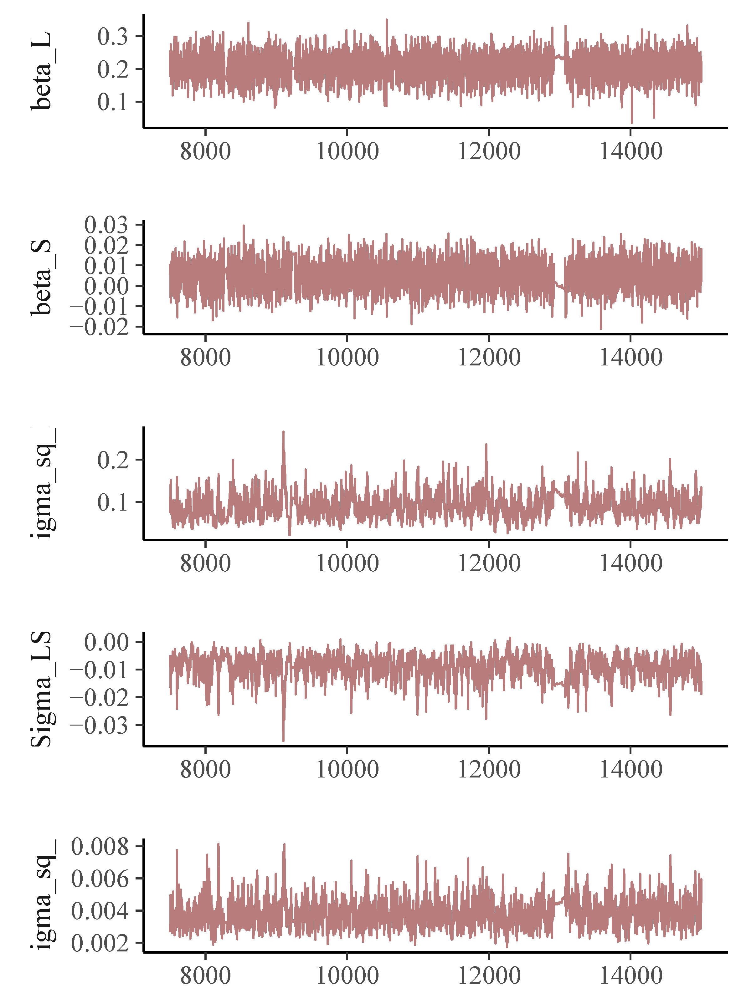
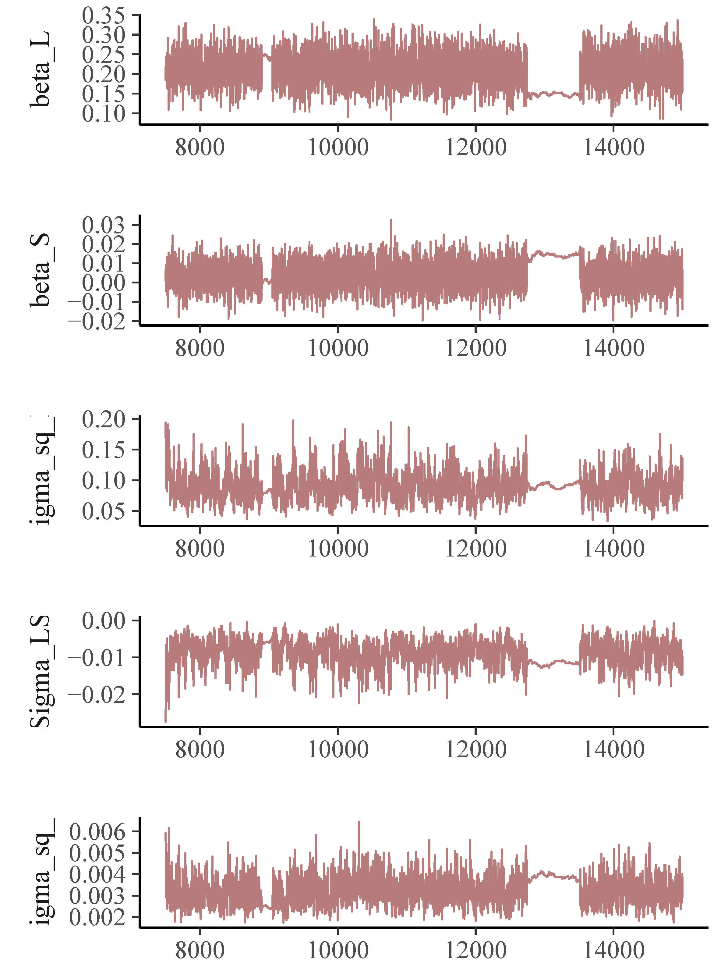
The trajectory plot for the memory scores (Figure 1) suggests a linear growth curve structure for the development of memory abilities. In the Bayesian estimation of DOME GCM, we assign a normal prior for the location vector $\boldsymbol {\beta }$, an inverse-gamma distribution for the measurement error variance $\sigma _\epsilon ^2$, and an inverse-Wishart for the random effect covariance $\Sigma $. For both the conditional median-based GCM and DOME GCM estimation, the total length of Markov chains is set as 15,000, with the first 7,500 draws being the burn-in period. Geweke statistics suggest that the Markov chains are stable after the burn-in period. The trace plots (Figures 2- 3) also suggest the convergence of the Markov chains.
The parameter estimates using the three methods are summarized in Table 3, and they differ a lot. The estimated rate of change $\hat {\beta }_S$ is 0.021 based on the traditional mean-based method. The estimates coming from the robust methods are much smaller, 0.003 from the conditional median-based approach, and 0.005 from the DOME growth curve modeling. Also, the $95\%$ credible interval of $\hat {\beta }_S$ from traditional mean-based method is $[0.001, 0.042]$, suggesting the memory ability for the investigated population (median age of the group is 55) has a significant increasing trend. In contrast, the intervals produced by the two robust methods all cover zero, which is more reasonable and interpretable as most participants in the dataset are elderly. The parameter estimates from the two robust methods are similar. Based on our simulation results, when there is no leverage observation in the dataset, conditional median-based method and DOME growth curve modeling are expected to give similar results. That is most likely the case in this illustrative example. The difference between traditional method and the robust methods is the result of the presence of outliers in the dataset. As suggested in our simulation study, we should generally trust the results from DOME. The results from DOME show that the initial median memory ability is about 0.203. The credible intervals indicate that there are significant between-subject differences in both initial ability and the change over time. The covariance between the two random effects is -0.009, and is significantly different from 0, meaning that a higher initial level is associated with a slower rate of change in general.
| Estimate | SE | CI | Geweke Statistic | |
Mean GCM | ||||
| $\beta _{L}$ | 0.186 | 0.037 | [0.114, 0.258] | |
| $\beta _{S}$ | 0.021 | 0.011 | [0.001, 0.042] | |
| $\sigma _{L}^{2}$ | 0.374 | 0.036 | [0.304, 0.444] | |
| $\sigma _{LS}$ | -0.014 | 0.008 | [-0.031, 0.002] | |
| $\sigma _{S}^{2}$ | 0.016 | 0.004 | [0.001, 0.023] | |
Median GCM
| ||||
| $\beta _{L}$ | 0.217 | 0.039 | [0.139, 0.289] | -0.337 |
| $\beta _{S}$ | 0.003 | 0.007 | [-0.010, 0.017] | 0.709 |
| $\sigma _{L}^{2}$ | 0.089 | 0.023 | [0.052, 0.140] | -0.707 |
| $\sigma _{LS}$ | -0.009 | 0.003 | [-0.016, -0.003] | 1.001 |
| $\sigma _{S}^{2}$ | 0.003 | 0.001 | [0.002, 0.005] | -0.603 |
Double Median GCM
| ||||
| $\beta _{L}$ | 0.203 | 0.038 | [0.127, 0.278] | 0.108 |
| $\beta _{S}$ | 0.005 | 0.007 | [-0.008, 0.018] | 0.465 |
| $\sigma _{L}^{2}$ | 0.093 | 0.028 | [0.050, 0.158] | -0.790 |
| $\sigma _{LS}$ | -0.009 | 0.004 | [-0.019, -0.003] | 0.287 |
| $\sigma _{S}^{2}$ | 0.004 | 0.001 | [0.002, 0.006] | -0.573 |
Growth curve modeling based on conditional medians has been developed to disentangle the influence of data contamination. In this paper, we developed a DOME GCM, a double medians based structure, to handle both outliers and leverage observations in longitudinal data. A simulation study was conducted to compare the numerical performances of traditional mean-based growth curve modeling, a median-based growth curve modeling, as well as the proposed DOME growth curve modeling. Results showed that when data were normally distributed, the three methods performed equally well. When data contain outliers but not leverage observations, the median-based method and DOME growth curve modeling yielded similar parameter estimates, which were less biased and more efficient than those from traditional growth curve modeling. When leverage observations existed, DOME growth curve modeling outperformed the other two approaches, providing much less biased parameter estimates. We therefore recommend to use DOME growth curve modeling in general as it can effectively handle both leverage observations and outliers.
As pointed out in Tong and Zhang (2017), outliers and leverage observations are equally likely to exist in samples in practice, but they affect model estimation differently. Although various methods have been developed to identify outliers and leverage observations separately, the accuracy and effectiveness of those methods were not guaranteed, especially in longitudinal studies. Tong and Zhang (2017) suggested that a final detection decision should rely on a combination of multiple methods. Our work in this paper indirectly provided an approach to imply whether data contain leverage observations or not, by comparing the estimation results from the median-based growth curve modeling and the DOME growth curve modeling. If their results greatly deviate from each other, we can conclude that leverage observations exist.
Note that estimations of the random effects parameters (e.g., $\sigma _S^2$) are not as good as those for the fixed effects (e.g., $\beta _S$) in general. This is consistent with the literature; namely, although the median has a higher breakdown point of 50%, it can be less efficient than the mean under some conditions. Thus, we need to carefully examine the estimated random effects parameters to determine whether there are significant between-subject variations in the within-subject change. One alternative approach is to extend the current approach based on conditional medians to approaches based on conditional quantiles. Such extension is natural with the assistance of asymmetric Laplace distributions, and we would be able to investigate the change pattern at different quantile levels inferring between-subject differences without investigating the random effects parameters.
In this study, we evaluated the performance of DOME growth curve modeling when data were contaminated. We want to point out that the data distribution nonnormality may be due to data contamination or nonnormal population distributions. Although we expect that the developed DOME GCM should still perform well when population distributions are nonnormal, it worths systematically assessing the effectiveness of DOME GCM and compare it with existing robust methods in future research.
Missing data in longitudinal data are inevitable, yet the conditional median based approaches have not been applied to analyze data with missing values. Since Bayesian methods were used for the DOME GCM estimation, multiple imputations can be automatically implemented and missing values can be accommodated relatively easily. We will extend the developed method to handle ignorable and non-ignorable missing data in future research.
This paper is based upon work supported by the National Science Foundation under grant no. SES-1951038.
Cho, H., Hong, H. G., & Kim, M.-O. (2016). Efficient quantile marginal regression for longitudinal data with dropouts. Biostatistics, 17, 561–575. doi: https://doi.org/10.1093/biostatistics/kxw007
Depaoli, S., Liu, H., & Marvin, L. (2021). Parameter specification in bayesian cfa: An exploration of multivariate and separation strategy priors. Structural Equation Modeling: A Multidisciplinary Journal, 0(0), 1-17. doi: https://doi.org/10.1080/10705511.2021.1894154
Galvao, A. F., & Poirier, A. (2019). Quantile regression random effects. Annals of Econometrics and Statistics, 134, 109–148. (DOI: 10.15609/annaeconstat2009.134.0109) doi: https://doi.org/10.15609/annaeconstat2009.134.0109
Geraci, M. (2014). Linear quantile mixed models: the lqmm package for laplace quantile regression. Journal of Statistical Software, 57, DOI: 10.18637/jss.v057.i13. doi: https://doi.org/10.18637/jss.v057.i13
Geweke, J. (1992). Evaluating the accuracy of sampling-based approaches to calculating posterior moments. In J. M. Bernado, J. O. Berger, A. P. Dawid, & A. F. M. Smith (Eds.), Bayesian statistics 4 (pp. 169–193). Oxford, UK: Clarendon Press.
Huang, Y. (2016). Quantile regression-based Bayesian semiparametric mixed-effects modelsfor longitudinal data with non-normal, missing and mismeasured covariate. Journal ofStatistical Computation and Simulation, 86, 1183–1202. (DOI: 10.1080/00949655.2015.1057732) doi: https://doi.org/10.1080/00949655.2015.1057732
Koenker, R. (2004). Quantile regression for longitudinal data. Journal of Multivariate Data Analysis, 91, 74–89. doi: https://doi.org/10.1016/j.jmva.2004.05.006
Koenker, R., & Bassett, G. (1978). Regression quantiles. Econometrica, 46, 33–50. doi: https://doi.org/10.2307/1913643
Kozubowski, T. J., & Podgorski, K. (2000). A multivariate and asymmetric generalization of laplace distribution. Computational Statistics, 15, 531–540. (DOI: 10.1007/PL00022717) doi: https://doi.org/10.1007/pl00022717
Lange, K. L., Little, R. J. A., & Taylor, J. M. G. (1989). Robust statistical modeling uisng the t distribution. Journal of the Americal Statistical Association, 84(408), 881–896. doi: https://doi.org/10.2307/2290063
Lu, Z., & Zhang, Z. (2014). Robust growth mixture models with non-ignorable missingness: Models, estimation, selection, and application. computational statistics and data analysis. Computational Statistics and Data Analysis, 71, 220–240. doi: https://doi.org/10.1016/j.csda.2013.07.036
McArdle, J. J., & Nesselroade, J. R. (2014). Longitudinal data analysis using structural equation models. American Psychological Association. doi: https://doi.org/10.1037/14440-000
Micceri, T. (1989). The unicorn, the normal curve, and other improbable creatures. Psychological Bulletin, 105(1), 156–166. doi: https://doi.org/10.1037/0033-2909.105.1.156
Pendergast, J. F., & Broffitt, J. D. (1985). Robust estimation in growth curve models. Communications in Statistics: Theory and Methods, 14, 1919–1939. doi: https://doi.org/10.1080/03610928508829021
Reich, B. J., Bondell, H. D., & J., W. H. (2010). Flexible bayesian quantile regression for independent and clustered data. Biostatistics, 11, 337–352. doi: https://doi.org/10.1093/biostatistics/kxp049
Rosseel, Y. (2012). lavaan: An R package for structural equation modeling. Journal of Statistical Software, 48, 1–36. Retrieved from http://www.jstatsoft.org/v48/i02/
Salthouse, T. A. (2014). Correlates of cognitive change. Journal of Experimental Psychology: General, 143, 1026–1048. doi: https://doi.org/10.1037/a0034847
Salthouse, T. A. (2018). Why is cognitive change more negative with increased age? Neuropsychology, 32, 110–120. doi: https://doi.org/10.1037/neu0000397
Singer, J. M., & Sen, P. K. (1986). M-methods in growth curve analysis. Journal of Statistical Planning and Inference, 13, 251–261. doi: https://doi.org/10.1016/0378-3758(86)90137-0
Smith, L. B., Fuentes, M., Gordon-Larsen, P., & Reich, B. J. (2015). Quantile regression for mixed models with an application to examine blood pressure trends in china. The Annals of Applied Statistics, 9, 1226–1246. doi: https://doi.org/10.1214/15-aoas841
Stan Development Team. (2019). RStan: the R interface to Stan. Retrieved from http://mc-stan.org/ (R package version 2.19.2)
Tong, X., Zhang, T., & Zhou, J. (2021). Robust bayesian growth curve modelling using conditional medians. British Journal of Mathematical and Statistical Psychology, 74(2), 286-312. doi: https://doi.org/10.1111/bmsp.12216
Tong, X., & Zhang, Z. (2012). Diagnostics of robust growth curve modeling using student’s t distribution. Multivariate Behavioral Research, 47, 493–518. doi: https://doi.org/10.1080/00273171.2012.692614
Tong, X., & Zhang, Z. (2017). Outlying observation diagnostics in growth curve modeling. Multivariate Behavioral Research, 52, 768–788. doi: https://doi.org/10.1080/00273171.2017.1374824
Yuan, K.-H., & Bentler, P. M. (1998a). Structural equation modeling with robust covariances. Sociological Methodology, 28, 363–396. doi: https://doi.org/10.1111/0081-1750.00052
Yuan, K.-H., & Bentler, P. M. (2001). Effect of outliers on estimators and tests in covariance structure analysis. British Journal of Mathematical and Statistical Psychology, 54, 161–175. doi: https://doi.org/10.1348/000711001159366
Zhang, H., Huang, Y., Wang, W., Chen, H., & Langland-Orban, B. (2019). Bayesian quantile regression-based partially linear mixed-effects joint models for longitudinal data with multiple features. Statistical Methods in Medical Research, 28, 569–588. (DOI: 10.1177/0962280217730852) doi: https://doi.org/10.1177/0962280217730852
Zhong, X., & Yuan, K.-H. (2010). Weights. In N. J. Salkind (Ed.), Encyclopedia of research design (pp. 1617–1620). Thousand Oaks, CA: Sage.
Zhong, X., & Yuan, K.-H. (2011). Bias and efficiency in structural equation modeling: Maximum likelihood versus robust methods. Multivariate Behavioral Research, 46, 229–265. doi: https://doi.org/10.1080/00273171.2011.558736
The “rstan” package (Stan Development Team, 2019) is used in our study. Below we provide the annotated R code for the real data analysis.
DOME<-"
data{
  int<lower=0> N;
  int<lower=0> T;
  vector[N*T] X;
  vector[N*T] y;

  // fixed inv_gamma parameter, prior of epsilon variance
  real shape;
  real inv_scale;

  // beta prior information, the global slope&intercept
  vector[2] beta_0;
  cov_matrix[2] Var_beta0;

  // hyper parameter’s value for Var_b
  cov_matrix[2] Var_b0;
}

transformed data{
  int len;
  len = N*T;
}

parameters{
  real<lower=0> sigma; //epsilon variance
  vector<lower=0>[len] v; // data augmentation, represent
                            // Laplace epsilon in expo
  vector<lower=0>[N] vb; // data augmentation, MLD b

  vector[2] beta;
  vector[2] b_star[N];

  cov_matrix[2] Var_b;
  cov_matrix[2] Var_beta;
}

transformed parameters{
  vector[len] mu;
  vector[len] sigma_y;
  vector[N] vb_root;

  vb_root = sqrt(vb);

  for(i in 1:N){
    for(j in 1:T){
      mu[T*(i-1)+j] = beta[1] + b_star[i,1]*vb_root[i] +
        (beta[2] + b_star[i, 2]*vb_root[i]) * X[T*(i-1)+j];
    }
  }

  sigma_y = sqrt(sigma*v);
}

model{
  // model
  y ~ normal(mu, sigma_y);

  // data augmentation
  sigma ~ inv_gamma(shape, inv_scale);
  v ~ exponential(1);
  vb ~ exponential(1);

  // priors
  beta ~ multi_normal(beta_0, Var_beta);
  // b_star * sqrt(vb) is b, written this way to vectorize
  b_star ~ multi_normal([0, 0], Var_b);
  Var_beta ~ inv_wishart(3, Var_beta0);
  Var_b ~ inv_wishart(3, Var_b0);
}
"
#load VCAP data and prepare intial values for MCMC
y<-as.vector(y)
X<-as.vector(time)
N<-length(y)/5
lm_est<-lm(y~X)
beta_0<-c(lm_est$coefficients[1],lm_est$coefficients[2])
Var_beta0<-matrix(c(0.5,0,0,0.1),ncol = 2)
Var_b0<-matrix(c(0.5,0,0,0.1),ncol = 2)
dat<-list(N=N, T=T, y=y, X=X, beta_0=beta_0, shape=0.1,
   inv_scale=0.1, Var_beta0=Var_beta0, Var_b0=Var_b0)
v_initial<-rep(1,N*T)
vb_initial<-rep(1,N)
b_initial<-matrix(rep(0, N*2), N, 2)
intial<-list(list(sigma=runif(1,0.5,2), beta=beta_0,
    b=b_initial,  v=v_initial, vb=vb_initial,
    Var_beta=Var_beta0, Var_b=Var_b0))

#fit the DOME model using rstan package
fit_DOME<-stan(model_code=double_quantile, model_name="DOME",
  init=intial, pars=c("beta","Var_b"), data=dat, iter=15000,
  chains=1)
summary(fit_DOME)$summary

//check convergence via geweke test
content<-extract(fit_double_median)
geweke.diag(content$beta[,1])$z
geweke.diag(content$beta[,2])$z
geweke.diag(content$Var_b[, 1, 1])$z
geweke.diag(content$Var_b[, 1, 2])$z
geweke.diag(content$Var_b[, 2, 2])$z

#draw traceplot for MCMC, serving as reference for convergence
color_scheme_set(’mix-blue-red’)
mcmc_trace(fit_DOME,
    pars = c("beta[1]","beta[2]", "Var_b[1,1]", "Var_b[1,2]",
    "Var_b[2,2]"), facet_args = list(ncol = 1,
    strip.position = "left"), iter1 = 7500)


