Keywords: Structural equation modeling · Bayesian analysis · Inverse Wishart prior · Informative prior · Convergence diagnostics
Structural equation modeling (SEM) is widely used to analyze multivariate data with complex structures in behavioral and social sciences, due to its ability to identify relationships among unobserved latent variables using the observed data (e.g., P. Bentler & Dudgeon, 1996; Bollen, 1989; Jöreskog, 1978; Lee, 2007; MacCallum & Austin, 2000). In a typical SEM model, manifest variables, latent variables, and measurement error can be analyzed simultaneously (e.g., Anderson & Gerbing, 1988; Yuan, Kouros, & Kelley, 2008). The family of SEMs contains a large variety of well-known models such as path analysis models (e.g., Boker & McArdle, 2005; Yuan et al., 2008), confirmatory factor models (e.g., Jöreskog, 1969), and growth curve models (e.g., Grimm, Steele, Ram, & Nesselroade, 2013; McArdle & Nesselroade, 2003). One primary purpose of fitting an SEM model is to explain the covariance structure among variables, either latent or manifest. Such a covariance structure is depicted by parameters in the hypothetical model such as factor loadings, path coefficients, factor covariance matrices, and residual variances.
Bayesian methods are increasingly used in estimating SEMs (e.g. Lee, 2007; Palomo, Dunson, & Bollen, 2007; Van de Schoot, Winter, Ryan, Zondervan-Zwijnenburg, & Depaoli, 2017). The seminal work by Lee (2007) laid the ground for Bayesian SEM. Guo, Zhu, Chow, and Ibrahim (2012) used Bayesian Lasso for model regularization. Zhang, Lai, Lu, and Tong (2013) introduced a robust Bayesian method to estimate growth curve models. Wang, Feng, and Song (2016) employed the Bayesian method in estimating quantile SEMs. Muthen and Asparouhov (2012) proposed to use small variance priors to approximate parameters typically specified to be 0 in the frequentist framework. The increasing popularity of Bayesian methods first benefits from the computer hardware development that renders sampling techniques such as Markov Chain Monte Carlo (MCMC) samplers (Gelfand & Smith, 1990). It is also because of the many beneficial features of Bayesian statistics (Van de Schoot et al., 2017). For example, it is possible to incorporate prior information into the estimation process in data analysis, which has the analogous contribution of extra data and is particularly useful when the sample size is small where the maximum likelihood (ML) method meets troubles to converge (e.g., P. M. Bentler & Yuan, 1999). It can also be computationally tractable even for very complex models (e.g., Muthen & Asparouhov, 2012). In addition, it is especially flexible to handle missing data and latent variables using data augmentation techniques (e.g., Z. Lu, Zhang, & Lubke, 2011; Van Dyk & Meng, 2001; Zhang & Wang, 2012). Moreover, it treats model parameters as random variables with a more intuitive interpretation (Van de Schoot et al., 2017). Because of the increasing popularity of Bayesian statistical inference, the software has also been developed to facilitate the use of Bayesian SEM such as the R package blavaan (Merkle & Rosseel, 2015) and Mplus (Muthen & Asparouhov, 2012).
Despite the many advantages, the burden of using Bayesian SEM is also discussed (e.g., MacCallum, Edwards, & Cai, 2012). A common criticism on Bayesian statistics is the use of priors. First, it can be difficult to specify priors and risky to use default priors in software (Liu, Depaoli, & Marvin, 2022; Smid, McNeish, Miočević, & van de Schoot, 2019). In an SEM, there are many parameters including factor loadings, factor covariance matrix, unique factor variances, regression paths, and other parameters. Selecting priors for all those parameters can be tedious. Although default priors are provided in most existing software, their influences are still not well understood by many applied researchers, especially for complex models and/or small sample size studies (Depaoli, Liu, & Marvin, 2021; Smid et al., 2019). Second, the use of informative priors can significantly affect parameter estimates and Bayesian inference. In order to reduce the influence of priors and obtain objective inference, Jeffreys prior has been developed (Jeffreys, 1961). However, the derivation of Jeffreys prior is not straightforward and therefore convenient priors such as univariate and multivariate normal, Gamma, and Wishart priors are often used in practice (e.g., Lee & Song, 2012; Song & Lu, 2010; Zhang, Hamagami, Lijuan Wang, Nesselroade, & Grimm, 2007; Zhang et al., 2013). Third, some researchers have argued that informative priors should be used to fully take advantage of Bayesian inference (e.g., Z.-H. Lu, Chow, & Loken, 2016; Muthen & Asparouhov, 2012). However, the specification of such priors is even more delicate. Another concern is the use of Markov chain Monte Carlo (MCMC) techniques. The convergence diagnostics of the Markov chains are required and can be very challenging. The dependence among the Markov samples often suggests a long chain to provide reliable inferences. Therefore, the specification of priors and the diagnostics of convergence have become two major obstacles for the adoption of Bayesian SEM in practice. Although some existing software has implemented Bayesian MCMC techniques, it might not work well with the default settings for all models.
The objective of this paper is to present an alternative Bayesian approach to SEM that specifies prior distributions under a unified framework for all covariance structures. Rather than specifying priors on individual model parameters \(\boldsymbol {\theta }\), this approach specifies a multivariate prior distribution directly on the saturated population covariance matrix \(\mathbf {\Sigma }\). Random draws from the posterior distribution of the population covariance matrix are then fitted to the covariance structure to obtain posterior distributions of model parameters.
Compared to the existing procedures for Bayesian SEM, the newly proposed procedure has two distinct features. First, priors are only required for the population covariance matrix and there is no need to specify a prior for each individual model parameter such as factor loadings and residual variances. This substantially reduces the work for researchers, especially novel users of Bayesian methods, conducting a Bayesian SEM analysis. Inverse-Wishart priors have been adopted for the covariance matrix parameter in most of the existing Bayesian analyses (e.g., Grimm, Kuhl, & Zhang, 2013; Liu, Zhang, & Grimm, 2016; Pan, Song, Lee, & Kwok, 2008; Zhang, 2021; Zhang et al., 2007, 2013). In the current study, we also use Inverse-Wishart priors becasue it is not only computationally convenient but also practically meaningful. The prior information conveyed by an Inverse Wishart prior IW(\(m,{\bf V}\)) is the same as “additional” data with the sample size \(m\) and the sum of squares \(\bf V\). As a result, we are able to control the amount of prior information nested in the prior by adjusting the values of hyper-parameters of an Inverse-Wishart distribution. Second, the posterior samples of model parameters \(\boldsymbol {\theta }\) are independently and identically distributed. This is because the posterior distribution of the population covariance matrix is a marginal distribution and has a closed form. Thus, independent covariance matrices can be sampled from the posterior distribution directly. And so are the \(\bf \boldsymbol {\theta }'s\) mapped from them. Because every obtained sample is from its posterior distribution, it is not necessary to have a burn-in period and conduct convergence diagnostics. Because of the independence of samples, relatively fewer samples are needed to obtain reliable inferences compared to the conventional MCMC procedures.
The rest of this paper is organized as follows. We first provide a brief introduction to both structural equation modeling and Bayesian statistical inference.We then present our new approach to Bayesian SEM. The use of prior distributions, types of points estimates, and credible intervals are described. After that, we evaluate the performance and illustrate the application of the new procedure using a confirmatory factor model. Finally, we conclude the paper with discussions and future directions.
In this section, we provide a brief review of SEM and Bayesian inference in the aim to explain some notations used in the rest of the paper. More details can be found in the seminal works such as Gelman et al. (2013), Kruschke (2011), Lee (2007) and Lee and Song (2012).
A classical SEM contains two components: a measurement model and a structure model. Using the LISREL (Jöreskog & Sörbom, 1993) notations, it can be represented as follows, \begin {equation} \begin {split} {\bf x} = & \boldsymbol {\Lambda }\begin {bmatrix}\boldsymbol {\eta }\\ \boldsymbol {\xi } \end {bmatrix}+\varepsilon \\ {\bf \boldsymbol {\eta }} = & {\bf B}\boldsymbol {\eta }+\boldsymbol {\Gamma }\boldsymbol {\xi }+\boldsymbol {\delta } \end {split} \end {equation} where \(\boldsymbol {\eta }\) and \(\boldsymbol {\xi }\) are latent dependent (endogenous) and independent (exogenous) variables; \(\bf x\) is a vector of their indicators; \(\boldsymbol {\Lambda }\) is a factor loading matrix; \(\bf B\) and \(\boldsymbol {\Gamma }\) are two coefficient matrices to represent the relationship among latent dependent variables and between latent independent and latent dependent variables, respectively; and \(\boldsymbol {\epsilon }\) a vector of unique factors and \(\boldsymbol {\delta }\) represents the residuals of the structure model. The elements of \(\boldsymbol {\varepsilon }\) are independent of the elements in \(\boldsymbol {\delta }\), but the elements in \(\boldsymbol {\delta }\) are allowed to be correlated with each other as in the original LISREL model. For convenience, let \(\boldsymbol {\Psi }\) be the covariance matrix of \(\boldsymbol {\varepsilon }\) , \(\boldsymbol {\Phi }\) be the covariance matrix of various latent independent variables so that \(\text {cov}(\boldsymbol {\xi })=\boldsymbol {\Phi }\), and \(\mathbf {\Theta }=\text {cov}(\boldsymbol {\delta })\). We denote all the unknown parameters as \(\boldsymbol {\theta }\) that consists of factor loadings \(\boldsymbol {\Lambda }\), path coefficients \(\bf B\) and \(\boldsymbol {\Gamma }\), as well as \(\boldsymbol {\Phi }\) and \(\mathbf {\Theta }\). The model implied covariance matrix \(\Sigma (\boldsymbol {\theta })\) is a function of the unknown parameters \(\boldsymbol {\theta }\). In order to estimate the parameter \(\boldsymbol {\theta }\), both maximum likelihood (ML) estimation and Bayesian estimation methods can be used.
Following the tradition in structural equation modeling, the observed variable \(X\) is assumed to follow a multivariate normal distribution. When the covariance structure is of primary interests, the following discrepancy function is usually minimized to obtain the maximum likelihood estimates of \(\boldsymbol {\theta }\) \begin {equation} F_{ML}=\log |\mathbf {\Sigma }(\boldsymbol {\theta })|+\text {tr}(\mathbf {S}\mathbf {\Sigma }^{-1}(\boldsymbol {\theta }))-\log |{\mathbf {S}}|-p\label {eq:F_ML} \end {equation} where \(p\) is the number of manifest variables and \(\bf S\) is the sample covariance matrix as defined previously. Newton-types of algorithms are often employed to get ML estimates, which we refer to as \(\hat {\boldsymbol {\theta }}_{ML}\) in this study.
In Bayesian statistical inference, the model parameter \(\boldsymbol {\theta }\) is not a fixed number, but a random variable following a probability distribution. The joint distribution of data \(\bf X\) and model parameters \(\boldsymbol {\theta }\) is \[ P({\bf X},\boldsymbol {\theta })=P({\bf X}|\boldsymbol {\theta })P(\boldsymbol {\theta }), \] from which we can obtain the posterior distribution of \(\boldsymbol {\theta }\) conditional on \(n\) independent observations on \(\bf X\) : \({\bf x}_{1},{\bf x}_{2},\cdots ,{\bf x}_{n}\), \begin {equation} P(\boldsymbol {\theta }|{\bf x}_{1},\cdots ,{\bf x}_{n})=\frac {\Pi _{i=1}^{n}P({\bf x}_{i}|\boldsymbol {\theta })P(\boldsymbol {\theta })}{\Pi _{i=1}^{n}\int _{\boldsymbol {\theta }}P({\bf x}_{i},\boldsymbol {\theta })d\boldsymbol {\theta }}.\label {eq:bays-1} \end {equation} Here, \(P(\boldsymbol {\theta }|{\bf x}_{1},\cdots ,{\bf x}_{n})\) is called the posterior distribution of \(\boldsymbol {\theta }\) given data, and \(\Pi _{i=1}^{n}P({\bf x}_{i}|\boldsymbol {\theta })\) is the likelihood function, which is a function of \(\boldsymbol {\theta }.\) The term \(P(\boldsymbol {\theta })\) represents the prior distribution of \(\boldsymbol {\theta },\) which summarizes the information on the model parameters based on the prior knowledge. Because the denominator of the above equation is the marginal distribution of data and it is a constant with respect to model parameters \(\boldsymbol {\theta },\) we use \(P({\bf X})\) to represent it for convenience. The posterior distribution is then
where the symbol \(\propto \) means that a constant for scaling is removed. The posterior distribution itself is the combination of the likelihood function and the prior.
In SEM, there are latent variables involved. To obtain Bayesian inference, the data augmentation technique is usually adopted (Rubin, 1987; Tanner & Wong, 1987). Instead of working on the posterior marginal distribution of the unknown parameters, one could choose to work on the joint posterior distribution of unknown parameters and latent variables. For instance in a LISREL model, the joint posterior distribution is as follows \begin {equation} \begin {split} P(\boldsymbol {\Lambda },{\bf B},\boldsymbol {\Gamma },\boldsymbol {\Phi },\mathbf {\Theta },\sigma _{k}^{2},\boldsymbol {\eta },\boldsymbol {\xi }|& {\bf x}_{1},{\bf x}_{2},\cdots ,{\bf x}_{n}) \nonumber \\ \propto & P({\bf x}_{1},{\bf x}_{2},\cdots ,{\bf x}_{n}|\boldsymbol {\Lambda },{\bf B},\boldsymbol {\Gamma },\boldsymbol {\Phi },\mathbf {\Theta },\sigma _{k}^{2},\boldsymbol {\eta },\boldsymbol {\xi })\nonumber \\ & \times P(\boldsymbol {\Lambda },{\bf B},\boldsymbol {\Gamma },\boldsymbol {\Phi },\mathbf {\Theta },\sigma _{k}^{2},\boldsymbol {\eta },\boldsymbol {\xi })\nonumber \\ = & P({\bf x}_{1},{\bf x}_{2},\cdots ,{\bf x}_{n}|\boldsymbol {\Lambda },\sigma _{k}^{2},\boldsymbol {\eta },\boldsymbol {\xi })P(\boldsymbol {\eta }|\boldsymbol {\xi },{\bf B},\boldsymbol {\Gamma },\mathbf {\Theta })\nonumber \\ & \times P(\boldsymbol {\xi }|\boldsymbol {\Phi })P(\boldsymbol {\Lambda },{\bf B},\boldsymbol {\Gamma },\boldsymbol {\Phi },\mathbf {\Theta },\sigma _{k}^{2},k=1,\cdots ,p) \end {split} \end {equation} with \(P(\boldsymbol {\Lambda },{\bf B},\boldsymbol {\Gamma },\boldsymbol {\Phi },\mathbf {\Theta },\sigma _{k}^{2})\) being the joint prior distribution of unknown parameters. The adoption of such a technique does not only make the inference on model parameters easier analytically, but also provides Bayesian inference on latent variables directly.
In most existing Bayesian SEM studies, independent priors are used (e.g., Lee, 2007; Muthen & Asparouhov, 2012; Zhang et al., 2013) such that \begin {equation} P(\boldsymbol {\Lambda },{\bf B},\boldsymbol {\Gamma },\boldsymbol {\Phi },\mathbf {\Theta },\sigma _{k}^{2})=P(\boldsymbol {\Lambda })P({\bf B})P(\boldsymbol {\Gamma })P(\boldsymbol {\Phi })P(\mathbf {\Theta })P(\sigma _{k}^{2},k=1,\cdots ,p) \end {equation} For example, the following are the types of priors used as the default priors in the existing software such as Mplus and blavaan,
\begin {equation} \begin {split} \sigma _{k}^{2} & \sim \text {Inverse Gamma}(\alpha _{0k},\beta _{0k})\nonumber \\ \boldsymbol {\Lambda }_{k} & \sim \text {N}(\Lambda _{0k},H_{0k})\nonumber \\ {\bf B}_{k} & \sim \text {N}(B_{0k},J_{0k})\nonumber \\ \boldsymbol {\Gamma }_{k} & \sim \text {N}(\gamma _{0k},K_{0k})\\ \boldsymbol {\Phi } & \sim \text {IW}(T_{0},\beta _{0})\nonumber \\ \mathbf {\Theta } & \sim \text {IW}(R_{0},\rho _{0})\nonumber \end {split} \end {equation}
in which \(\sigma _{k}^{2}\) is the error variance of the \(k\)th observed variable;\(\boldsymbol {\Lambda }_{k},{\bf B}_{k},\boldsymbol {\Gamma }_{k}\) are the \(k\)th row of the factor loadings and path coefficients matrices, respectively; and \(\alpha _{0k},\beta _{0k},\Lambda _{0k},H_{0k},B_{0k},J_{0k},\gamma _{0k},K_{0k},T_{0},\beta _{0},R_{0}\), and \(\rho _{0}\) are the hyper-parameters of the prior distributions, whose values are designated based on the prior information.
To obtain samples from the posterior distribution, Markov Chain Monte Carlo (MCMC) iterative procedures such as Gibbs samplers are used in existing Bayesian SEM. With the given starting values \(\boldsymbol {\Lambda }^{0},{\bf B}^{0},\boldsymbol {\Gamma }^{0},\boldsymbol {\Phi }^{0},\mathbf {\Theta }^{0},(\sigma _{k}^{2})^{0},\)\((\boldsymbol {\eta }^{0},\boldsymbol {\xi }^{0})\), at \(j\)th iteration, sample
In SEM, the above conditional posterior distributions very often do not have analytically closed forms. Obtaining samples from the conditional distributions can be very complex and sampling schemes, such as the Metropolis–Hastings algorithms, are usually used within each step to draw samples from the conditional posterior distributions. Let \(\boldsymbol {\theta }\) be the vector of all model parameters; by repeating the above Gibbs procedure \(B\) times, where \(B\) is usually a large number, we will obtain a chain of posterior samples \(\boldsymbol {\theta }^{1},\boldsymbol {\theta }^{2},\cdots ,\boldsymbol {\theta }^{t},\cdots ,\)\(\boldsymbol {\theta }^{B}\).
Convergence diagnostics of the Markov chains are required in Bayesian analysis (e.g., Brooks & Roberts, 1998). This is because only the part of chains that has reached the stationary status would be representative of the posterior distribution. However, the diagnostics logically cannot guarantee representativeness. In addition, the successive draws by MCMC are correlated. Although the existence of auto-correlations does not necessarily mean bad point estimates, but correlated samples provide much less information than the same amount of uncorrelated ones. Higher auto-correlations usually suggest that longer chains are needed to have reliable inferences.
To summarize, in conventional Bayesian SEM, priors are specified on individual unknown parameters. MCMC procedures are used to obtain samples from the posterior distributions of model parameters. Convergence diagnostics of the Markov chains are required. Athough these can be done by software through default settings, it might lead to serious problems if researchers are not familiar with Bayesian methods. Hence, it is still not easy to conduct Bayesian SEM in general.
In this work we propose a different framework for Bayesian SEM. In this approach, a prior distribution is imposed on the space of saturated covariance matrices: \[ \mathbf {\Sigma }\sim \pi (\mathbf {\Sigma }) \] The choice of prior distribution \(\pi \) will be discussed shortly. As usual, the observations are assumed to independently follow a multivariate normal distribution. This implies \[ \mathbf {S}|\mathbf {\Sigma }\sim \mathrm {W}(\mathbf {\Sigma }/(n-1),(n-1)) \] where \(n\) is sample size and \(\mathbf {S}\) is the usual unbiased estimator of \(\mathbf {\Sigma }\).
It should be noted that the parameters in the covariance structure are not explicit in the formulation above; rather, they are considered implicit functions of variances and covariances in \(\mathbf {\Sigma }\): \[ \boldsymbol {\theta }^{*}=\textbf {argmin}\ F_{ML}(\mathbf {\Sigma },\mathbf {\Sigma }(\boldsymbol {\theta })) \] In addition, the discrepancy between the true population covariance matrix \(\mathbf {\Sigma }\) and the model implied covariance matrix \(\mathbf {\Sigma }^{*}=\mathbf {\Sigma }(\boldsymbol {\theta }^{*})\) is also a function of \(\mathbf {\Sigma }\): \[ F^{*}=\min _{\theta }F_{ML}(\mathbf {\Sigma },\mathbf {\Sigma }(\boldsymbol {\theta }))=F_{ML}(\mathbf {\Sigma },\mathbf {\Sigma }(\boldsymbol {\theta }^{*})) \]
The Wishart likelihood function of \(\mathbf {\Sigma }\) is given by \[ L(\mathbf {\Sigma }|\mathbf {S})\propto |\mathbf {\Sigma }|^{-n/2}\exp [-\frac {1}{2}\text {tr}(n\mathbf {S}\mathbf {\Sigma }^{-1})] \]
The posterior distribution is therefore \begin {equation} \pi (\mathbf {\Sigma }|\mathbf {S})\propto |\mathbf {\Sigma }|^{-n/2}\exp [-\frac {1}{2}\text {tr}(n\mathbf {S}\mathbf {\Sigma }^{-1})]\pi (\mathbf {\Sigma }). \end {equation} Many different priors can be used for \(\mathbf {\Sigma }\), this study focuses on the use of Jeffreys prior and the inverse Wishart prior.
Jeffreys prior (e.g., Gelman et al., 2013; Jeffreys, 1946) is a type of noninformative prior, for it does not incorporate extra information other than that from the data to the posterior distribution. For a model with a vector of parameters \(\boldsymbol {\zeta }\), its Jeffreys prior is defined through \begin {equation} \pi _{J}(\boldsymbol {\zeta })\propto \sqrt {\text {det}(\mathcal {I}(\boldsymbol {\zeta }))} \end {equation} where \(\mathcal {I}(\boldsymbol {\zeta })\) is the Fisher-information matrix. A Wishart likelihood is thus \begin {equation} \pi _{J}(\Sigma )=|\Sigma |^{-(p+1)/2} \end {equation} where \(p\) is the number of variables. This prior distribution was firstly developed by Jeffreys (1961) for \(p=1,2\), and later was generalized to arbitrary \(p\) (e.g., Geisser, 1965; Geisser & Cornfield, 1963; Villegas, 1969).
With the Jeffreys prior, the posterior distribution of \(\Sigma \) is
which is an Inverse Wishart (IW) distribution with degrees of freedom \(n\) and scale matrix \(n\mathbf {S}\), denoted as IW(\(n\),\(n\mathbf {S}\)) in this study.
The Inverse Wishart prior is a conjugate prior and is widely used in practice. The Inverse Wishart prior IW(\(m\),\(\mathbf {V}\)) has the following probability density function, \begin {equation} P(\Sigma |\mathbf {V},m)=\frac {|{\bf V}|^{m/2}}{2^{mp/2}\Gamma _{p}(\frac {m}{2})}|\Sigma |^{-\frac {m+p+1}{2}}\exp [-\frac {1}{2}\text {tr}({\bf V}\Sigma ^{-1})].\label {eq:inverse wishart} \end {equation} Note that with Jeffreys prior, the posterior distribution of the population covariance matrix is an Inverse Wishart distribution with the degrees of freedom being the sample size \(n\) and the scale matrix being the sums of squares \(n\mathbf {S}\). Comparing the form in Eqn (10) to that in Eqn (??), we notice the use of an Inverse Wishart prior IW(\(m\), \(\bf V\)) in an analysis is theoretically equivalent to provide \(m\) additional observations with sums of squares \(\bf V\) to the estimation of \(\Sigma \).
With the Inverse Wishart prior IW(\(m\),\(\mathbf {V}\)), the posterior distribution is also an Inverse Wishart distribution with the following kernel,
Thus it is the Inverse Wishart distribution IW(\(n+m,n\mathbf {S}+{\bf V}\)) with the degrees of freedom \(n+m\) and the scale matrix \(n\mathbf {S}+{\bf V}.\) Note that if we set \(\mathbf {V}=m\mathbf {S}\), then the prior represents \(\frac {100m}{n}\%\) of information of the data. Therefore, the amount of information in the prior can be easily quantified.
The posterior mean and mode are \(\frac {n\mathbf {S}+{\bf V}}{n+m-p-1}\) and \(\frac {n\mathbf {S}+{\bf V}}{n+m+p+1}\), respectively. For a fixed \(m\), both the posterior mean and mode as well as the sample covariance matrix \(\bf S\) will converge to the population covariance matrix \(\Sigma \) asymptotically. Thus, when the sample size is large, all three estimates \(\mathbf {S}\), \(\frac {n\mathbf {S}+{\bf V}}{n+m-p-1}\), and \(\frac {n\mathbf {S}+{\bf V}}{n+m+p+1}\) are similar. For a given \(n\), a larger \(m\) indicates that the prior influences the posterior distribution more.
In the existing Bayesian SEMs using an Inverse Wishart prior, the scale matrix \(\bf V\) is often chosen to be an identical matrix \(\bf I\). However, we could change the Inverse Wishart prior to an informative prior by using a specific scale matrix \({\bf V}.\) For instance, if we know the estimated sums of squares from another study, we can use it as our scale matrix in the Inverse Wishart prior. In addition, if one does not want to use prior information, one can set \(m=0\) and \({\bf V}={\bf 0}\). Note that the density function is not proper any more but the prior becomes the Jeffreys prior. In this sense, the Jefferys prior can be regarded as a special case of Inverse Wishart prior. Hence, in the rest of the paper, we only focus on the Inverse Wishart prior. Thus, the posterior distribution of the population covariance parameter is an inverse-Wishart distribution IW(\(n+m,n{\bf S}+{\bf V}\)).
With the posterior distribution of \(\Sigma \), i.e., IW(\(n+m,n{\bf S}+{\bf V}\)), we can further get a posterior distribution of model parameters. Let \(g\) be a function that maps a \(\Sigma \) to a \(\boldsymbol {\theta }_{\Sigma }\). Among the so many possible candidates, we define \(g({\bf \Sigma })\) as the \(\boldsymbol {\theta }\) that minimizes the distance between \(\Sigma (\boldsymbol {\theta })\) and \(\Sigma ,\) \begin {equation} \boldsymbol {\theta }_{\Sigma }=g(\Sigma )=\text {argmin}(\log |\Sigma (\boldsymbol {\theta })|+\text {tr}(\Sigma \Sigma ^{-1}(\boldsymbol {\theta }))-\log |\Sigma |)\label {eq:distance function} \end {equation} This step is analogous to the maximum likelihood (ML) estimation of SEM models, in which the sample covariance matrix \(\mathbf {S}\) is used as the estimate of the population covariance matrix \(\Sigma \). However, in Bayesian SEM, the population covariance matrix \(\Sigma \) is a random variable and can take values from the space \(\Omega _{\Sigma }.\) We therefore obtain a \(\boldsymbol {\theta }_{\Sigma }\) for a covariance matrix from the space \(\Omega _{\Sigma }.\)
By aplplying the mapping function \(g(\cdot )\) to the posterior distribution \(P(\Sigma |{\bf S})\), we could get a posterior distribution of \(\boldsymbol {\theta }\) called \(P(\boldsymbol {\theta }|{\bf S})\). Although we do not know the exact form of \(P(\boldsymbol {\theta }|{\bf S}),\)we could draw samples from it. To do so, we first drawn \(B\) independent samples of \(\Sigma \) denoted by \(\Sigma _{1},\Sigma _{2},\cdots ,\Sigma _{B}\) from \(P(\Sigma |{\bf S}).\) We then map each of such \(\Sigma _{b}\)s to \(\boldsymbol {\theta }_{b}\)s using the function \(g\) defined in (11).
With \(B\) samples \(\boldsymbol {\theta }_{1},\boldsymbol {\theta }_{2},\cdots ,\boldsymbol {\theta }_{B}\) obtained using the procedure described above, an estimate of posterior mean, called \(\bf \boldsymbol {\theta }\)-mean, is defined as the average of samples of \(\boldsymbol {\theta },\)
\begin {equation} \hat {\boldsymbol {\theta }}_{mean}=\frac {1}{B}\sum _{b=1}^{B}\boldsymbol {\theta }_{b}. \end {equation}
In addition to the \(\boldsymbol {\theta -}\)mean estimate, there are some other parameter estimates of practical interest. Depending on how the estimates of the population covariance matrix is constructed from its posterior distribution, we can have different forms of estimates as discussed below.
In Bayesian inference, the maximum a posteriori (MAP) estimate is of great interest, because it is the mode of a posterior distribution. With an Inverse Wishart prior IW(\(m,\text {{\bf V}}\)), the posterior mode of \(\Sigma \) is \(\Sigma _{mode}\)=\(\frac {nS+{\bf V}}{m+n+p+1}\). We then find its corresponding \(\boldsymbol {\theta }\) using Equation (11). The resulted \(\boldsymbol {\theta }\) is an estimate for the parameter \(\boldsymbol {\theta }\) and is called \(\Sigma \)-mode estimate in this study.
Similarly, we can also get the posterior mean of \(\Sigma \), \(\Sigma _{mean}=\frac {ns+{\bf V}}{m+n-p-1}\) and then finds out its corresponding \(\boldsymbol {\theta }.\)We will call it the \(\Sigma \)-mean estimate in the rest of \( \)this study. It is interesting to note that when the IW(\({\bf V=0},m=p+1\)), the \(\Sigma _{mean}\) is the same as the sample covariance matrix and \(\Sigma -\)mean estimate will concide the ML estimates of the model parameters.
Besides the point estimates, the posterior credible intervals can also be formed using the posterior samples \(\boldsymbol {\theta }_{b},b=1,\ldots B\). For each element \(\theta \) in the vector of parameters \(\boldsymbol {\theta }\) and a desired level \(\alpha \) between 0 and 1, the \(100 {\alpha }\%\) HPD credible interval is denoted by \([L_{\alpha },U_{\alpha }]\) as the one with smallest width among all the intervals containing \(\alpha \) proportion of samples.
So far, we have explained how to specify priors on the population covariance parameter, how to obtain posterior samples for model parameters \(\boldsymbol {\boldsymbol {\theta }}\). To obtain posterior statistics, we introduced three point estimates and the HPD credible intervals. Since the proposed approach specifies prior on the population covariance matrix, we call it “Covariance matrix prior Bayesian SEM (CP-BSEM)” in contrast to the traditional Bayesian SEM approaches (T-BSEM)
The CP-BSEM approach has several distinct features from the T-BSEM method. The first one is the prior specification. While using the CP-BSEM approach, we specify a prior on the population covariance matrix parameter \(\Sigma \). The posterior distributions of model parameters are transformed from the posterior distribution of the population covariance matrix \(P(\Sigma |data)\). We can notice that the CP-BSEM approach reduces the burden of specifying priors and posterior diagnostics.
However, an essential question that arises is whether the CP-BSEM approach can lead to comparable posterior inference on \(\boldsymbol {\theta }\) as to a T-BSEM approach. While using a T-BSEM approach, an implict assumption is that the model is a correct model and there is no model misfit. In the following, we will show that the CP-BSEM is coupling to a T-BSEM approach with a certain prior specification when the model is a true model.
Let \(P_{\text {IW}}(\Sigma )\) be the density function of the Inverse Wishart prior \(\text {IW}(m,{\bf V})\) for the population covariance matrix parameter \(\Sigma \) and \(g(\cdot )\) be a function that maps a \(\Sigma \) to a \(\boldsymbol {\theta }\) as defined by Equation (11). When applying the \(g\) function to the entire space of \(\Sigma \), i.e., \(\Omega _{\Sigma },\)with the probability density function \(P_{\text {IW}}(\Sigma )\), we could get a probability distribution function on \(\boldsymbol {\theta }\). Specifically, \[ g:\big (\Omega _{\Sigma },P_{\text {IW}}\big )\rightarrow \big (\Omega _{\boldsymbol {\theta }},P_{\text {IW}}(\Sigma (\boldsymbol {\theta }))\big ) \] where \(P_{\text {IW}}(\Sigma (\boldsymbol {\theta }))\) is the probability distribution on model parameters \(\boldsymbol {\theta }\) that is transformed from \(P_{\text {IW}}\) by the mappling function \(g(\cdot )\).
Let \(P(\Sigma |data)\) be the posterior distribution and it is still an Inverse Wishart distribution \(\text {IW}(m+n,n{\bf S}+{\bf V}).\) We can transform it to a distribution on \(\boldsymbol {\theta }\), named as \(P_{\Sigma }(\boldsymbol {\theta }|data)\), using the mapping function \(g(\cdot )\), \begin {equation} \begin {split} P_{\Sigma }(\boldsymbol {\theta }|data) & =P(g^{-1}(\boldsymbol {\theta })|data)\\ & =P(\Sigma |data)\\ & =P(data|g(\Sigma ))P_{\text {IW}}(\Sigma )\\ & =P(data|\Sigma \boldsymbol {(\boldsymbol {\theta })})P_{\text {IW}}(\Sigma (\boldsymbol {\theta })) \end {split} \end {equation} where \(P(data|\Sigma (\boldsymbol {\theta }))\) is the likehood for given \(\boldsymbol {\theta }\) and \(P_{\text {IW}}(\Sigma (\boldsymbol {\theta }))\) is a prior distribution on model parameter \(\boldsymbol {\theta }.\) Therefore, the distribution on \(\boldsymbol {\theta }\) transformed from the posterior distribution of \(\Sigma \) is actually a posterior distribution of \(\boldsymbol {\theta }\) with the given prior distribution \(P_{\text {IW}}(\Sigma (\boldsymbol {\theta }))\) using the T-BSEM approach.
As discussed above, the proposed CP-BSEM approach can be coupled to a T-BSEM, therefore it can achieve comparable inference with the T-BSEM approach. Moreover, it eases up the burden of prior specification and has better interpretation of the prior information, and it does not need posterior diagnosis.
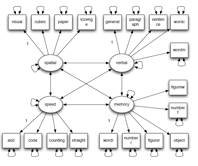
To show how to use the newly proposed CP-BSEM approach, we analyzed the data from Holzinger and Swineford (1939), which includes measures on 19 tests from 145 eighth grade students in the Grant-White School and 156 students from the Pasteur School. As an illustration, we focus on the analysis of the data from the Grant-White School. The 19 tests were intended to measure four attributes: spatial ability, verbal ability, process speed, and working memory. Therefore, we fitted a four-factor confirmatory factor model shown in Figure 1. In identifying the model, we fixed one factor loading for each factor to be 1 and freely estimated the factor variances and covariances as shown in the path diagram.
For the purpose of illustration, we analyzed the data using two different priors. The first one is a noninformative prior IW(\(19,{\bf I}\)). The second prior was an informative prior formed based on the data from the Pasteur school. With the noninformative prior, the posterior distribution for the population covariance matrix is IW(\(145+19,145\mathbf {S}_{GW}+{\bf I}\)), with \(\mathbf {S}_{GW}\) being the sample covariance matrix of the data from Grant-White School.
The informative prior distribution was specified as the posterior distribution obtained based on the data from the Pasteur School with \(156\) participants. In the analysis of the Pasterur School data, suppose the same noninformative prior IW(\(19,{\bf I}\)) was used, which led to the posterior distribution IW(156+19,156\(\mathbf {S}_{P}+{\bf I}\)), with \(\mathbf {S}_{P}\) being the sample covariance matrix of the data from Pasteur School. Using it as the prior distribution for the Grant-White school data analysis, we redid the analysis of the Grant-White School data and the resulting posterior distribution is IW(\(145+156+19,145\mathbf {S}_{GW}+156\mathbf {S}_{P}+{\bf I}\)). Note that in practical data analysis, the raw data to form the prior are often not available. Therefore, the current way for incorporating prior information is even more practical to substantive researchers.
The model parameter estimates using the two priors based on \(\Sigma \)-mean together with the \(95\%\) HPD credible intervals and the width of the intervals are summarized in Table 1. Note that the unique factor variances are not reported to save space. Clearly, all the \(95\%\) HPD intervals excluded \(0\) and, therefore, one may conclude all the parameters were statistically significant from 0 in the frequentist hypothesis testing sense. The parameter estimates obtained using noninformative and informative priors were quite different. In addition, the HPD intervals using the informative prior were narrower consistently than those from using the noninformative prior. According to our simulation, when the IW(\(19,{\bf I}\)) was used, the estimates should be close to MLE. Therefore, the difference was because of the use of prior information in the Bayesian estimation process. The choice between the two sets of estimates depends on whether we wanted to use the prior information or not. If the inference was supposed to be based on only the data from the Grant-White School, the noninformative prior should be used. If the inference was designed to also combine the information from the Pasteur School, the informative prior should be adopted. This empirical example illustrated that it is possible either to use or not to use prior information.
| Noninformative Prior | Informative Prior | ||||||||||||||
| ML | \(\boldsymbol {\theta }_{\boldsymbol {\Sigma }_{mode}}\) | \(\boldsymbol {\theta }_{\boldsymbol {\Sigma }_{mean}}\) | \(\boldsymbol {\theta }_{mean}\) | \(95\%\) CI | W | \(\boldsymbol {\theta }_{\boldsymbol {\Sigma }_{mode}}\) | \(\boldsymbol {\theta }_{\boldsymbol {\Sigma }_{mean}}\) | \(\boldsymbol {\theta }_{mean}\) | \(95\%\) CI | W | |||||
| visual | 0.689 | 0.612 | 0.691 | 0.688 | 0.513 | 0.866 | 0.352 | 0.708 | 0.757 | 0.755 | 0.62 | 0.889 | 0.269 | ||
| cubes | 0.477 | 0.423 | 0.479 | 0.476 | 0.292 | 0.659 | 0.368 | 0.435 | 0.465 | 0.466 | 0.322 | 0.605 | 0.283 | ||
| paper | 0.541 | 0.48 | 0.543 | 0.541 | 0.365 | 0.719 | 0.354 | 0.474 | 0.506 | 0.504 | 0.373 | 0.636 | 0.264 | ||
| lozenge | 0.674 | 0.598 | 0.676 | 0.675 | 0.507 | 0.856 | 0.348 | 0.623 | 0.665 | 0.666 | 0.528 | 0.804 | 0.277 | ||
| general | 0.805 | 0.715 | 0.808 | 0.806 | 0.674 | 0.957 | 0.283 | 0.793 | 0.847 | 0.846 | 0.748 | 0.954 | 0.206 | ||
| paragrap | 0.817 | 0.725 | 0.819 | 0.817 | 0.679 | 0.961 | 0.282 | 0.784 | 0.838 | 0.838 | 0.736 | 0.942 | 0.207 | ||
| sentence | 0.834 | 0.74 | 0.837 | 0.834 | 0.702 | 0.978 | 0.276 | 0.824 | 0.881 | 0.881 | 0.782 | 0.988 | 0.207 | ||
| wordc | 0.693 | 0.615 | 0.696 | 0.695 | 0.551 | 0.849 | 0.298 | 0.686 | 0.733 | 0.733 | 0.63 | 0.844 | 0.214 | ||
| wordm | 0.840 | 0.745 | 0.843 | 0.842 | 0.707 | 0.987 | 0.281 | 0.812 | 0.868 | 0.868 | 0.767 | 0.974 | 0.207 | ||
| add | 0.649 | 0.576 | 0.651 | 0.65 | 0.453 | 0.844 | 0.39 | 0.588 | 0.628 | 0.626 | 0.484 | 0.766 | 0.282 | ||
| code | 0.694 | 0.616 | 0.696 | 0.691 | 0.52 | 0.858 | 0.338 | 0.708 | 0.757 | 0.756 | 0.629 | 0.888 | 0.259 | ||
| counting | 0.697 | 0.619 | 0.699 | 0.699 | 0.524 | 0.877 | 0.353 | 0.596 | 0.637 | 0.637 | 0.496 | 0.778 | 0.282 | ||
| straight | 0.745 | 0.662 | 0.748 | 0.747 | 0.566 | 0.93 | 0.364 | 0.63 | 0.673 | 0.674 | 0.537 | 0.812 | 0.275 | ||
| wordr | 0.515 | 0.457 | 0.516 | 0.515 | 0.314 | 0.707 | 0.394 | 0.549 | 0.587 | 0.585 | 0.446 | 0.722 | 0.276 | ||
| numberr | 0.516 | 0.458 | 0.518 | 0.517 | 0.342 | 0.698 | 0.356 | 0.497 | 0.531 | 0.53 | 0.395 | 0.669 | 0.274 | ||
| figurer | 0.595 | 0.528 | 0.597 | 0.597 | 0.415 | 0.78 | 0.365 | 0.58 | 0.619 | 0.617 | 0.477 | 0.764 | 0.286 | ||
| object | 0.627 | 0.556 | 0.629 | 0.626 | 0.443 | 0.81 | 0.367 | 0.578 | 0.618 | 0.616 | 0.476 | 0.754 | 0.279 | ||
| numberf | 0.648 | 0.575 | 0.65 | 0.647 | 0.463 | 0.83 | 0.367 | 0.538 | 0.575 | 0.574 | 0.44 | 0.714 | 0.274 | ||
| figurew | 0.482 | 0.428 | 0.484 | 0.481 | 0.303 | 0.666 | 0.363 | 0.461 | 0.493 | 0.492 | 0.352 | 0.629 | 0.277 | ||
| spatial \(\sim \)verbal | 0.594 | 0.594 | 0.594 | 0.593 | 0.425 | 0.732 | 0.307 | 0.504 | 0.504 | 0.502 | 0.369 | 0.616 | 0.248 | ||
| spatial \(\sim \) speed | 0.583 | 0.583 | 0.582 | 0.577 | 0.336 | 0.771 | 0.435 | 0.469 | 0.469 | 0.467 | 0.302 | 0.619 | 0.316 | ||
| spatial \(\sim \) memory | 0.635 | 0.635 | 0.635 | 0.632 | 0.409 | 0.804 | 0.395 | 0.499 | 0.499 | 0.495 | 0.336 | 0.644 | 0.308 | ||
| verbal \(\sim \) speed | 0.467 | 0.467 | 0.467 | 0.463 | 0.276 | 0.615 | 0.339 | 0.464 | 0.464 | 0.462 | 0.339 | 0.576 | 0.237 | ||
| verbal \(\sim \) memory | 0.496 | 0.497 | 0.497 | 0.496 | 0.319 | 0.647 | 0.328 | 0.347 | 0.347 | 0.346 | 0.206 | 0.474 | 0.268 | ||
| speed \(\sim \) memory | 0.605 | 0.605 | 0.605 | 0.599 | 0.405 | 0.76 | 0.355 | 0.552 | 0.552 | 0.55 | 0.408 | 0.675 | 0.267 | ||
The purpose of the simulation study are twofold. First, we would like to evaluate the performance of the CP-BSEM approach. We will compare the three types of point estimates in terms of how well they could recover the true parameter values. We will also evaluate the HPD credible intervals to see whether it has good coverage rates. Second, we will compare the CP-BSEM approach with two other competing approaches: The ML approach and the T-BSEM approach. Therefore, we will also report the results of the ML method and the C-BSEM approach with default settings, which are implemented in R packages lavaan (Rosseel, Oberski, Byrnes, Vanbrabant, & Savalei, 2013) and blavaan (Merkle & Rosseel, 2015).
The simulation study is designed based on the 4-factor confirmatory factor model with 19 normally distributed indicators as used in the empirical data analysis presented later. Let \(Z\) be the normally distributed random vectors of \(19\) variables with mean \(\boldsymbol {0}\) and the four latent factors be \(\mathbf {f}=(f_{1},f_{2},f_{3},f_{4})'\). The factor model is \begin {align} Z & =\mathbf {\Lambda }\mathbf {f}+\boldsymbol {\varepsilon } \end {align}
where \(\mathbf {\Lambda }\) is a 19 by 4 factor loading matrix, and \(\boldsymbol {\varepsilon }=(\varepsilon _{1},\varepsilon _{2},\cdots ,\varepsilon _{19})'\) is the unique factor score. The factor loading matrix has the following form, \[ \mathbf {\Lambda }=\begin {pmatrix}\boldsymbol {\lambda _{1}} & \boldsymbol {0} & \boldsymbol {0} & \boldsymbol {0}\\ \boldsymbol {0} & \boldsymbol {\lambda _{2}} & \boldsymbol {0} & \boldsymbol {0}\\ \boldsymbol {0} & \boldsymbol {0} & \boldsymbol {\lambda _{3}} & \boldsymbol {0}\\ \boldsymbol {0} & \boldsymbol {0} & \boldsymbol {0} & \boldsymbol {\lambda _{4}} \end {pmatrix} \] with \(\boldsymbol {\lambda _{1}}=(1,.693,.785,.978)'\) , \(\boldsymbol {\lambda }_{2}=(1,1.015,1.036,0.861,1.043)'\), \(\boldsymbol {\lambda _{3}}=(1,1.069, \\ 1.075, 1.149)'\), \(\boldsymbol {\lambda }_{4}=(1,1.004,1.156,1.218,1.259,0.936)'\). The covariance matrix of the latent factors is \[ \mathbf {\Phi }=\begin {pmatrix}.473 & .328 & .260 & .224\\ .328 & .646 & .243 & .205\\ .260 & .243 & .420 & .201\\ .224 & .205 & .201 & .264 \end {pmatrix}, \] and the uniqueness factor covariance matrix \(\mathbf {\Psi }\) is a diagonal matrix with diagonal elements (0.517, 0.763, 0.699, 0.537, 0.344, 0.325, 0.297, 0.511, 0.287, 0.570, 0.511, 0.505, 0.436, 0.726, 0.724, 0.637, 0.598, 0.572, 0.759). All parameter values are chosen to reflect the parameter estimates in the empirical data analysis.
Based on the population model, we generate \(1000\) data sets for each of the following sample sizes: 100, 150, 250, 300 and 500. Then, we fit the model to the generated data using ML, two-stage Bayesian, and traditional Bayesian methods. In the two-stage Bayesian method, the “noninformative” prior IW(\(19,\) \(\bf I\)) is used since we want to evaluate the parameter bias and estimation efficiency. In addition, \(10000\) covariance matrices are sampled independently from the posterior distribution of \(\Sigma \) to form the credible intervals. For traditional Bayesian estimates, the R package blavaan is used and the following default priors are adopted in the estimation: \begin {equation*} \begin {split} \text {factor loadings }\lambda _{j,k} & \overset {iid}{\sim }\text {N}(0,10^{4})\\ \text {factor covariance matrix }\Phi & \sim \text {IW}(5,{\bf I})\\ \text {unique factor variances }\sigma _{k}^{2} & \overset {iid}{\sim }\text {IG}(1,0.5) \end {split} \end {equation*} where \(\lambda _{j,k}\) represents the factor loading from the \(j\)th factor to the \(k\)th indicator; \(\sigma _{k}^{2}\) is the unique factor variance of the \(k\)th indicator. Finally, MLE is obtained using the R package lavaan.
To evaluate the performance of each method, we report the relative bias, coverage rates of the HPD credible intervals/confidence intervals, and mean squared errors for the model parameters.
Let \(\theta \) represent a parameter or its true value. The relative bias is defined as the percent ratio of the discrepancy between the estimate and the true value with respect to the true value of a parameter:
where \(\bar {\theta }\) is the average of the estimates in \(R\), which is 1000 successful replications in our simulation, \[ \bar {\theta }=\frac {1}{R}\sum _{r=1}^{R}\hat {\theta }_{r}. \] with \(\hat {\theta }_{r}\) denoting the parameter estimate in the \(r\)th replication.
The mean squared errors (MSE) are calculated as, \begin {equation} \begin {split} \text {MSE}_{\theta } & =\frac {1}{R}\sum _{r=1}^{R}(\hat {\theta }_{r}-\theta )^{2}\\ & =\frac {1}{R}\sum _{r=1}^{R}(\hat {\theta }_{r}-\bar {\theta })^{2}+\frac {1}{R}\sum _{r=1}^{R}(\bar {\theta }-\theta )^{2} \end {split} \end {equation} which is the sum of the variance and squared biases of the parameter estimates.
The coverage rate of the \(95\%\) HPD credible interval for Bayesian and confidence interval for MLE represents the proportion of the intervals covering the true parameter value. Mathematically, if \([L_{0.95}^{r},U_{0.95}^{r}]\) is the interval in the \(r\)th replication, the coverage rate (CR) is calculated as \[ \text {CR}_{\theta }=\frac {1}{R}\sum _{r=1}^{R}I(\theta \in [L_{0.95}^{r},U_{0.95}^{r}]). \] where \(I(\cdot )\) is the index function with value 1 if the interval covers the true value and 0, otherwise. A CR around \(0.95\) implies that the defined 95% interval performs well.
We now present the results on relative biases, coverage rates, and mean squared errors from our simulation. There are 44 parameters grouped into three types – 15 factor loadings, 19 unique factor variances, and 10 factor covariances. Since we found that the influence of estimation methods on each type of parameters is similar, we only report the average relative biases, coverage rates, and mean squared errors for the three types of parameters to save space. For relative bias, we calculate the average based on the absolute values because bias can be positive or negative.
The average absolute relative biases for factor loadings, factor covariance matrix and unique factor variances are provided in Table 2. For the two-stage Bayesian, the three types of parameter estimates are presented. For the traditional Bayesian, the posterior mean and median are obtained using blavaan.
Overall, the bias decreased as the sample size increased for parameter estimates. For the factor loadings, the bias for \(\Sigma \)-mean estimates was small even when the sample size was 100 and was almost the same as the ML estimates. \(\mathbf {\boldsymbol {\theta }}\)-mean had larger bias than \(\Sigma \)-mean estimates but overall was better than the traditional method. Although \(\mathbf {\Sigma }\)-mode estimates had small bias for factor loadings but had large bias for factor covariance and unique factor variances. This indicates that in using the two-stage Bayesian for parameter estimates, either \(\Sigma \)-mean or \(\mathbf {\boldsymbol {\theta }}\)-mean estimates should be preferred.
Comparing the two-stage method with the traditional Bayesian method, it was clear that the two-stage method provided less biased parameter estimates using the chosen prior. This is because we had better control of the prior information in the two-stage method.
| CP-BSEM | T-BSEM | ||||||||
| N | ML | \(\Sigma \)-mode | \(\Sigma \)-mean | \(\mathbf {\theta }\)-mean | Mean | Median | |||
| Factor loading
| |||||||||
| 100 | 2.421 | 2.419 | 2.419 | 8.300 | 8.691 | 6.87 | |||
| 150 | 1.357 | 1.357 | 1.357 | 3.329 | 6.246 | 4.969 | |||
| 200 | 0.926 | 0.926 | 0.926 | 2.306 | 4.941 | 3.949 | |||
| 250 | 0.958 | 0.958 | 0.958 | 1.992 | 4.295 | 3.483 | |||
| 300 | 0.748 | 0.748 | 0.748 | 1.579 | 3.626 | 2.940 | |||
| 500 | 0.461 | 0.461 | 0.461 | 0.924 | 2.354 | 1.933 | |||
| Factor covariance | |||||||||
| 100 | 1.263 | 28.694 | 0.733 | 1.853 | 9.706 | 12.613 | |||
| 150 | 1.101 | 20.181 | 1.366 | 1.885 | 6.37 | 8.393 | |||
| 200 | 0.99 | 16.882 | 0.690 | 1.142 | 6.228 | 7.752 | |||
| 250 | 0.698 | 13.764 | 0.598 | 0.891 | 4.969 | 6.199 | |||
| 300 | 0.441 | 11.575 | 0.435 | 0.712 | 4.086 | 5.118 | |||
| 500 | 0.342 | 7.115 | 0.403 | 0.535 | 2.502 | 3.124 | |||
| Unique factor variance
| |||||||||
| 100 | 2.352 | 28.294 | 0.915 | 1.069 | 2.292 | 1.242 | |||
| 150 | 1.573 | 20.813 | 0.607 | 0.858 | 1.535 | 0.968 | |||
| 200 | 1.165 | 16.447 | 0.542 | 0.621 | 1.199 | 0.774 | |||
| 250 | 0.993 | 13.655 | 0.329 | 0.439 | 0.921 | 0.57 | |||
| 300 | 0.703 | 11.53 | 0.378 | 0.321 | 0.896 | 0.493 | |||
| 500 | 0.49 | 7.315 | 0.228 | 0.258 | 0.503 | 0.364 | |||
The mean squared errors for the parameters are provided in Table 3. Similar to the bias, the MSE also decreased as the sample size increased for all parameters regardless of the estimation methods. The mean squared errors were mostly comparable with two notable observations. First, the MSE for MLE and \(\Sigma \)-mean were almost identical. This again suggested the control of prior information. Second, the MSE from the traditional Bayesian method was smaller than MLE. This is because the use of the prior information. Therefore, in terms of both bias and MSE, the two-stage method has better control of the influence of the prior information.
| MSE\(\times 100\) | CP-BSEM | T-BSEM | ||||||
| N | ML | \(\Sigma \)-mode | \(\Sigma \)-mean | \(\mathbf {\theta }\)-mean | Mean | Median | ||
| Factor loading
| ||||||||
| 100 | 5.742 | 5.737 | 5.737 | 20.775 | 5.271 | 4.765 | ||
| 150 | 3.555 | 3.553 | 3.553 | 4.377 | 3.415 | 3.147 | ||
| 200 | 2.466 | 2.466 | 2.466 | 2.792 | 2.517 | 2.343 | ||
| 250 | 2.027 | 2.027 | 2.027 | 2.220 | 2.078 | 1.951 | ||
| 300 | 1.636 | 1.635 | 1.635 | 1.763 | 1.687 | 1.592 | ||
| 500 | 0.941 | 0.941 | 0.941 | 0.979 | 0.984 | 0.942 | ||
| Factor covariance | ||||||||
| 100 | 0.953 | 1.517 | 0.972 | 0.970 | 0.816 | 0.859 | ||
| 150 | 0.672 | 0.940 | 0.679 | 0.682 | 0.593 | 0.613 | ||
| 200 | 0.497 | 0.698 | 0.500 | 0.501 | 0.463 | 0.477 | ||
| 250 | 0.388 | 0.528 | 0.391 | 0.392 | 0.362 | 0.372 | ||
| 300 | 0.332 | 0.426 | 0.335 | 0.336 | 0.313 | 0.319 | ||
| 500 | 0.197 | 0.236 | 0.198 | 0.198 | 0.190 | 0.194 | ||
| Unique factor variance
| ||||||||
| 100 | 0.935 | 3.061 | 0.935 | 0.910 | 0.924 | 0.891 | ||
| 150 | 0.608 | 1.783 | 0.608 | 0.602 | 0.605 | 0.590 | ||
| 200 | 0.459 | 1.196 | 0.459 | 0.453 | 0.456 | 0.449 | ||
| 250 | 0.367 | 0.874 | 0.366 | 0.364 | 0.365 | 0.360 | ||
| 300 | 0.306 | 0.667 | 0.307 | 0.304 | 0.306 | 0.303 | ||
| 500 | 0.179 | 0.328 | 0.180 | 0.179 | 0.179 | 0.179 | ||
The coverage rates for model parameters are displayed in Table 4. Overall, the coverage rates were close to the nominal level 0.95 except for the factor covariances when the traditional Bayesian method was used.
| N | ML | CP-BSEM | T-BSEM | ||
| 100 | 94.29 | 95.21 | 94.43 | ||
| 150 | 94.43 | 95.03 | 94.48 | ||
| Factor loading | 200 | 94.85 | 95.03 | 94.54 | |
| 250 | 94.61 | 94.98 | 94.60 | ||
| 300 | 94.86 | 94.90 | 94.57 | ||
| 500 | 95.41 | 95.18 | 95.01 | ||
| 100 | 92.70 | 94.71 | 90.34 | ||
| 150 | 93.36 | 94.47 | 91.27 | ||
| Factor covariance | 200 | 93.41 | 94.33 | 91.30 | |
| 250 | 94.35 | 95.21 | 92.68 | ||
| 300 | 93.82 | 94.39 | 92.28 | ||
| 500 | 94.73 | 94.93 | 93.61 | ||
| 100 | 92.22 | 94.53 | 95.30 | ||
| 150 | 93.31 | 94.72 | 95.35 | ||
| Unique factor variance | 200 | 93.65 | 94.70 | 95.35 | |
| 250 | 93.87 | 94.52 | 94.97 | ||
| 300 | 94.10 | 94.67 | 95.08 | ||
| 500 | 94.46 | 94.86 | 95.18 | ||
In summary, our two-stage Bayesian method can obtain results similar to ML method by controlling the prior information. Comparing to the T-BSEM method, it also offers better control of prior information.
In traditional Bayesian SEM, a prior needs to be specified for each individual or individual set of model parameters. Due to the complexity of SEM models and the diverse features of different types of model parameters, specifying priors is not an easy task, especially if one would like to control or utilize prior information. To get parameter estimates, MCMC procedures are often used and the convergence diagnostics of MCMC samples are always required, which is usually hard for researchers conducting applied researches.
In the present study, an alternative Bayesian procedure, i.e., CP-BSEM, is proposed to assist researchers conducting Bayesian statistical inference of SEMs. It has several distinct benefits over the traditional Bayesian procedures. First, the prior information is only required for the population covariance matrix parameter \(\Sigma \). Using the Inverse Wishart prior, we can control the prior information ranging from noninformative to very informative. The information can be conveniently controlled by varying its degrees of freedom and scale matrix. For instance, when both the degrees of freedom and scale matrix are set at 0, it becomes the Jeffreys prior for covariance matrix analysis with normal data. Increasing the degrees of freedom and/or using a special scale matrix, we could make the Inverse Wishart prior informative. The amount of information can also be directly compared to the data at hand.
Unlike the traditional Bayesian SEM, the CP-BSEM procedure does not require convergence diagnostics. With the use of the Inverse Wishart prior, the posterior of the population covariance matrix still follows an Inverse Wishart distribution. Therefore, independently and identically distributed samples of covariance matrix can be drawn from the posterior distribution directly. The corresponding samples of parameter estimates are thus independently and identically distributed, too. Since the samples are identically distributed, convergence diagnostics are not needed any more. The independence among the samples enables us to use relatively fewer samples to get reliable inferences than the traditional Bayesian SEM.
Results from our simulation study show that the CP-BSEM procedure works well in estimating structural equation models in general. Among the three point estimates, the \(\Sigma \)-mean estimates, obtained by fitting the SEM model to the posterior mean of the covariance matrix, is recommended. They have ignoble relative biases (\(<5\%\)) with results close to MLE. In addition, the credible interval has good coverage rates. We also notice that the traditional Bayesian SEM had slightly smaller MSEs than our two-stage procedure and MLE. This is due to more prior information involved in their prior distributions. By changing the prior distribution, traditional Bayesian SEM can also reduce the influence of prior distributions. However, as we have pointed out, controlling the prior information in traditional Bayesian analysis can be difficult, especially for applied researchers.
Compared to the traditional Bayesian method, the performance of the CP-BSEM procedure is less affected by the model complexity. Because the prior information is put on the population covariance matrix, it is independent to the model structure. Therefore, we could extend our results to a more general SEM model.
The CP-BSEM procedure is flexible to control prior information. In our empirical example, we demonstrated the use of informative prior, which was the posterior distribution of the covariance matrix from another study, also an Inverse Wishart distribution. Hence, the CP-BSEM approach can be used to conduct meta-analysis by combining several related studies in the SEM framework. Instead of combing model parameter estimates of every single study, one could combine the covariance matrices of different studies, in which the posterior distribution of the previous study will work as the prior distribution in the new study. One immediate benefit is that the inference will focus on the overall covariance matrix, but not the individual model parameters in each study. As a result, it has special advantages in combining studies without a common model structure.
The CP-BSEM approach is closely related to the parametric bootstrap technique for SEM. Covariance matrices are drawn from its posterior distribution repeatedly, and samples of parameter estimates are obtained by minimizing the descrepancy between the model implied covariance matrix to the sampled covariance matrices. The HPD credible intervals formed based on the samples of model parameters are, therefore, have the similar meaning to the bootstrap confidence intervals. However, in bootstrap, no prior information is allowed but the CP-BSEM approach can easily utilize prior information. Therefore, it could be particularly useful, when the original data set has a small sample size and the actual model parameters estimates are hard to obtain.
Even with the advantages, we want to note that the CP-BSEM approach can still not replace the traditional Bayesian SEM. For example, currently, missing data and non-normal data cannot be handled yet. Therefore, to increase the impact of the CP-BSEM and to help the adoption of the Bayesian methods, the CP-BSEM approach can be expanded in the following aspects. First, the present version of CP-BSEM procedure focuses on SEMs without mean structures. Extending the method to include the mean structure can make it possible to conduct growth curve analysis and multiple group analysis. Second, how to handle missing data in the CP-BSEM procedure should be investigated. Third, ways should be evaluated to handle non-normal data in the CP-BSEM procedure. Fourth, in traditional Bayesian SEM, deviance information criterion and posterior predictive p-values have been used for model fit evaluation. They can also be incorporated in the CP-BSEM approach.
The study was supported by a grant from the Institute of Education Sciences (R305D210023).
Anderson, J., & Gerbing, D. W. (1988). Structural equation modeling in practice: A review and recommended two-step approach. Psychological Bulletin, 103(3), 411–423. doi: https://doi.org/10.1037/0033-2909.103.3.411
Bentler, P., & Dudgeon, P. (1996). Covariance structure analysis: Statistical practice, theory, and direction. Annual l Review of Psychology, 47(1), 563 –592. doi: https://doi.org/10.1146/annurev.psych.47.1.563
Bentler, P. M., & Yuan, K.-H. (1999). Structural equation modeling with small samples: Test statistics. Multivariate Behavioral Research, 34(2), 181–197. doi: https://doi.org/10.1207/S15327906Mb340203
Boker, S. M., & McArdle, J. J. (2005). Path analysis and path diagrams. Wiley StatsRef: Statistics Reference Online, 3, 1529 –1531. doi: https://doi.org/10.1002/9781118445112.stat06517
Bollen, K. (1989). Structure equations with latent variables. New York: Wiley.
Brooks, S. P., & Roberts, G. O. (1998). Convergence assessment techniques for markov chain monte carlo. Statistics and Computing, 8(4), 319–335. doi: https://doi.org/10.1023/A:1008820505350
Depaoli, S., Liu, H., & Marvin, L. (2021). Parameter specification in bayesian cfa: An exploration of multivariate and separation strategy priors. Structural Equation Modeling: A Multidisciplinary Journal, 28(5), 699–715. doi: https://doi.org/10.1080/10705511.2021.1894154
Geisser, S. (1965). Bayesian estimation in multivariate analysis. The Annals of Mathematical Statistics, 36(1), 150–159.
Geisser, S., & Cornfield, J. (1963). Posterior distributions for multivariate normal parameters. Journal of the Royal Statistical Society. Series B (Methodological), 368–376. doi: https://doi.org/10.1080/01621459.1990.10476213
Gelfand, A., & Smith, A. (1990). Sampling-based approaches to calculating marginal densities. Journal of the American Statistical Association, 85, 398–409. doi: https://doi.org/10.1080/01621459.1990.10476213
Gelman, A., Carlin, J. B., Stern, H. S., Dunson, D. B., Vehtari, A., & Rubin, D. B. (2013). (3rd ed.). CRC press Boca Raton, FL.
Grimm, K. J., Kuhl, A. P., & Zhang, Z. (2013). Measurement models, estimation, and the study of change. Structural Equation Modeling: A Multidisciplinary Journal, 20(3), 504–517. doi: https://doi.org/10.1080/10705511.2013.797837
Grimm, K. J., Steele, J. S., Ram, N., & Nesselroade, J. R. (2013). Exploratory latent growth models in the structural equation modeling framework. Structural Equation Modeling: A Multidisciplinary Journal, 20(4), 568–591. doi: https://doi.org/10.1080/10705511.2013.824775
Guo, R., Zhu, H., Chow, S.-M., & Ibrahim, J. G. (2012). Bayesian lasso for semiparametric structural equation models. Biometrics, 68(2), 567–577. doi: https://doi.org/10.1111/j.1541-0420.2012.01751.x
Holzinger, K. J., & Swineford, F. (1939). A study in factor analysis: the stability of a bi-factor solution. Supplementary Educational Monographs.
Jeffreys, H. (1946). An invariant form for the prior probability in estimation problems. In Proceedings of the royal society of london a: Mathematical, physical and engineering sciences (Vol. 186, pp. 453–461).
Jeffreys, H. (1961). Theory of probability. Jeffreys, H.: Oxford University Press.
Jöreskog, K. G. (1969). A general approach to confirmatory maximum likelihood factor analysis. Psychometrika, 34(2), 183 - 202. doi: https://doi.org/10.1007/BF02289343
Jöreskog, K. G. (1978). Structural analysis of covariance and correlation matrices. Psychometrika, 43, 443–477. doi: https://doi.org/10.1007/BF02293808
Jöreskog, K. G., & Sörbom, D. (1993). Lisrel 8: Structural equation modeling with the simplis command language. Scientific Software International.
Kruschke, J. K. (2011). Bayesian assessment of null values via parameter estimation and model comparison. Perspectives on Psychological Science, 6(3), 299–312. doi: https://doi.org/10.1177/1745691611406925
Lee, S.-Y. (2007). Structure equation modeling: A bayesian approach. John Wiley and Sons.
Lee, S.-Y., & Song, X.-Y. (2012). Basic and advanced bayesian structural equation modeling: With applications in the medical and behavioral sciences. John Wiley & Sons.
Liu, H., Depaoli, S., & Marvin, L. (2022). Understanding the deviance information criterion for sem: Cautions in prior specification. Structural Equation Modeling: A Multidisciplinary Journal, 29(2), 278–294. doi: https://doi.org/10.1080/10705511.2021.1994407
Liu, H., Zhang, Z., & Grimm, K. J. (2016). Comparison of inverse wishart and separation-strategy priors for bayesian estimation of covariance parameter matrix in growth curve analysis. Structural Equation Modeling: A Multidisciplinary Journal, 23(3), 354–367. doi: https://doi.org/10.1080/10705511.2015.1057285
Lu, Z., Zhang, Z., & Lubke, G. (2011). Bayesian inference for growth mixture models with latent class dependent missing data. Multivariate behavioral research, 46(4), 567–597. doi: https://doi.org/10.1080/00273171.2011.589261
Lu, Z.-H., Chow, S.-M., & Loken, E. (2016). Bayesian factor analysis as a variable-selection problem: Alternative priors and consequences. Multivariate Behavioral Research, 51(4), 519–539. doi: https://doi.org/10.1080/00273171.2016.1168279
MacCallum, R. C., & Austin, J. T. (2000). Applications of structural equation modeling in psychological research. Annual review of psychology, 51(1), 201–226. doi: https://doi.org/10.1146/annurev.psych.51.1.201
MacCallum, R. C., Edwards, M. C., & Cai, L. (2012). Hopes and cautions in implementing bayesian structural equation modeling. Psychological Methods, 17(3), 340-345. doi: https://doi.org/10.1037/a0027131
McArdle, J., & Nesselroade, J. (2003). Growth curve analysis in contemporary psychological research. Comprehensive handbook of psychology: Research methods in psychology, 2, 447 - 480. doi: https://doi.org/10.1002/0471264385.wei021
Merkle, E. C., & Rosseel, Y. (2018). blavaan: Bayesian structural equation models via parameter expansion. Journal of Statistical Software, 85(4), 340–345. doi: https://doi.org/10.18637/jss.v085.i04
Muthen, B., & Asparouhov, T. (2012). Bayesian structural equation modeling: A more flexible representation of substantive theory. Psychological Methods, 17(3), 313-335. doi: https://doi.org/10.1037/a0026802
Palomo, J., Dunson, D., & Bollen, K. (2007). Bayesian structural equation modeling. Handbook of latent variable and related models, 163-188. doi: https://doi.org/10.1016/B978-044452044-9/50011-2
Pan, J. H., Song, X. Y., Lee, S. Y., & Kwok, T. (2008). Longitudinal analysis of quality of life for stroke survivors using latent curve models. Stroke, 39(10), 2795–2802. doi: https://doi.org/10.1161/STROKEAHA.108.515460
Rosseel, Y., Oberski, D., Byrnes, J., Vanbrabant, L., & Savalei, V. (2013). lavaan: Latent variable analysis.[software]. URL http://CRAN. R-project. org/package= lavaan (R package version 0.5-14).
Rubin, D. B. (1987). The calculation of posterior distributions by data augmentation: Comment: A noniterative sampling/importance resampling alternative to the data augmentation algorithm for creating a few imputations when fractions of missing information are modest: The sir algorithm. Journal of the American Statistical Association, 82(398), 543–546. doi: https://doi.org/10.2307/2289457
Smid, S. C., McNeish, D., Miočević, M., & van de Schoot, R. (2019). Bayesian versus frequentist estimation for structural equation models in small sample contexts: A systematic review Structural Equation Modeling: A Multidisciplinary Journal, 27(1), 131–161. doi: https://doi.org/10.1080/10705511.2019.1577140
Song, X.-Y., & Lu, Z.-H. (2010). Semiparametric latent variable models with bayesian p-splines. Journal of Computational and Graphical Statistics, 19(3), 590–608. doi: https://doi.org/10.1198/jcgs.2010.09094
Tanner, M. A., & Wong, W. H. (1987). The calculation of posterior distributions by data augmentation. Journal of the American statistical Association, 82(398), 528–540. doi: https://doi.org/10.2307/2289457
Van de Schoot, R., Winter, S. D., Ryan, O., Zondervan-Zwijnenburg, M., & Depaoli, S. (2017). A systematic review of bayesian articles in psychology: The last 25 years. Psychological Methods, 22(2), 217–239. doi: https://doi.org/10.1037/met0000100
Van Dyk, D. A., & Meng, X.-L. (2001). The art of data augmentation. Journal of Computational and Graphical Statistics, 10(1), 1–50. doi: https://doi.org/10.1198/10618600152418584
Villegas, C. (1969). On the a priori distribution of the covariance matrix. The Annals of Mathematical Statistics, 40, 1098-1099. doi: https://doi.org/10.1214/aoms/1177697617
Wang, Y., Feng, X.-N., & Song, X.-Y. (2016). Bayesian quantile structural equation models. Structural Equation Modeling: A Multidisciplinary Journal, 23(2), 246–258. doi: https://doi.org/10.1080/10705511.2015.1033057
Yuan, K.-H., Kouros, C., & Kelley, K. (2008). Diagnosis for covariance structure models by analyzing the path. Structural Equation Modeling, 15, 564-602. doi: https://doi.org/10.1080/10705510802338991
Zhang, Z. (2021). A note on wishart and inverse wishart priors for covariance matrix. Journal of Behavioral Data Science, 1(2), 119–126. doi: https://doi.org/https://doi.org/10.35566/jbds/v1n2/p2
Zhang, Z., Hamagami, F., Lijuan Wang, L., Nesselroade, J. R., & Grimm, K. J. (2007). Bayesian analysis of longitudinal data using growth curve models. International Journal of Behavioral Development, 31(4), 374–383. doi: https://doi.org/10.1177/0165025407077764
Zhang, Z., Lai, K., Lu, Z., & Tong, X. (2013). Bayesian inference and application of robust growth curve models using student’s t distribution. Structural Equation Modeling: A Multidisciplinary Journal, 20(1), 47–78. doi: https://doi.org/10.1080/10705511.2013.742382
Zhang, Z., & Wang, L. (2012). A note on the robustness of a full bayesian method for nonignorable missing data analysis. Brazilian Journal of Probability and Statistics, 26(3), 244–264. doi: https://doi.org/10.1214/10-BJPS132