Keywords: Convergence diagnostics · Bayesian analysis · Gelman-Rubin diagnostic · Geweke diagnostic
In recent decades, Bayesian statistics have been widely used given the development of Markov chain Monte Carlo (MCMC) sampling techniques and the growth of computational power (e.g., Van de Schoot et al., 2017). They have been used in cognitive psychology (e.g., Lee, 2008), developmental psychology (e.g., Van de Schoot et al., 2014; Walker et al., 2007), social psychology (e.g., Marsman et al., 2017), and many other areas. In the Bayesian framework, parameters are treated as random variables. Thus, we need to specify prior distributions for unknown parameters and obtain their posterior distributions. A major challenge of Bayesian methods that has not yet been fully addressed is how we can appropriately evaluate the convergence of the random samples to the target posterior distributions and the convergence of posterior means to the target mean. With nonconverged results, researchers may obtain severely biased parameter estimates and misleading statistical inferences. Therefore, there is a critical need to develop keen diagnostic methods for appropriately assessing convergence.
In the Bayesian framework, an MCMC algorithm converges when it samples thoroughly and stably from a density. More specifically, a converged Markov chain should have two properties: stationarity and mixing. To claim convergence, Markov chains need to move around in the posterior density in an appropriate manner and to mix well throughout the support of the density. In other words, when there are multiple Markov chains supporting the same estimation, they should trace out a common distribution (Gelman et al., 2014).
Practically, the convergence of MCMC algorithms can be assessed by visual inspection (i.e., trace plots) as well as quantitative evaluation. Various quantitative methods have been proposed for assessing convergence. To name a few, there are Garren and Smith (2000), Gelman and Rubin (1992), Geweke (1992), Heidelberger and Welch (1983), Johnson (1996), Liu, Liu, and Rubin (1992), and Raftery and Lewis (1992). Among them, the Gelman and Rubin’s method and Geweke ’s method currently are the most commonly used diagnostics and are implemented in popular software and R packages. For example, Mplus (Muthén and Muthén, 2017), CODA (Plummer et al., 2015), and BUGS (Spiegelhalter et al., 1996) can implement the Gelman and Rubin’s diagnostic, and CODA can implement the Geweke ’s diagnostic. The Gelman and Rubin’s diagnostic requires multiple MCMC chains with different starting values, and potential scale reduction factor (PSRF) is used for assessing the convergence of chains for individual parameters. Brooks and Gelman (1998) further generalized the univariate PSRF to a multivariate scale reduction factor (MPSRF), which tests all the parameters’ convergences as a group. The Geweke’s diagnostic only requires one MCMC chain, therefore it is generally less time-consuming in calculation.
Several papers (Brooks and Roberts, 1998; Cowles and Carlin, 1996; El Adlouni et al., 2006) reviewed and/or compared different convergence diagnostics with hypothetical examples. The common conclusion from these papers is that no method can perform well in all cases, therefore they recommended a joint use of all diagnostics. The recommendation is constructive in ensuring convergence, but it may be overly conservative and infeasible in practice. First, there are more than 10 convergence diagnostics, not to mention that those diagnostics require the analyses in multiple software. Researchers rarely perform all diagnostics in one real data analysis. Second, the statistical performance (i.e., Type I error rate which is the probability of rejecting a true null hypothesis that assumes convergence, and Type II error rate which is the probability of not rejecting a false null hypothesis that assumes convergence) of the Gelman and Rubin’s and the Geweke’s methods has not yet been evaluated in simulation studies. Additionally, the performances of Gelman and Rubin’s and Geweke’s diagnostics were examined in relatively complex models, such as bimodal mixture of trivariate normals (Cowles and Carlin, 1996) and shifting level model (El Adlouni et al., 2006), in which the analytical forms were unknown or hard to access. As a consequence, the performance of these diagnostics when convergence is ensured (e.g., Type I error rates) is still unknown.
Besides the challenge of having too many convergence diagnostics, another challenge is that there are usually multiple parameters in one analysis. If we assess the convergence of Markov chains of each parameter, we face a multiple testing problem for the entire analysis. If no correction is applied and we claim that the convergence for the entire analysis is achieved when the convergence assessment for every parameter is passed, the Type I error rate at analysis level (i.e., analysis-wise Type I error rate) can be substantially inflated. For example, suppose that there are 20 independent parameters and we use the Geweke’s diagnostic where the Type I error rate per parameter is supposed to be 5%. The analysis-wise Type I error rate is then $1-0.95^{20}=0.642$, which is far above the intended level (i.e., 0.05) and implies that it is too easy to obtain a non-convergence conclusion using the Geweke’s diagnostic. Applying conventional multiple testing corrections such as the Bonferroni correction might help reduce the inflated Type I error rates. However, parameters usually are not independent, and as illustrated later, the cutoff value for the Geweke’s diagnostic is approximated, therefore the actual performance of multiple testing corrections remains an open question. In terms of the Gelman and Rubin’s diagnostic, its cutoff comes from researchers’ recommendation. The Type I error rate of the Gelman and Rubin’s method at the parameter level or the analysis level in the literature remains largely unknown.
Given the above-mentioned unanswered questions, we focus on Gelman and Rubin’s diagnostic, Brooks and Gleman’s multivariate diagnostic, and Geweke’s diagnostic, and aim to answer the following three questions in this paper:
(1) If we only choose one diagnostic, which one should we adopt? Even if no method performs well in all conditions, we would like to select the relatively better one. Type I error rate and Type II error rate are the two frequently used criteria for evaluating the performance of an analytic method. We therefore investigate this question based on these two criteria.
(2) In high dimension cases (i.e., the number of parameters is large), should we rely on the diagnostic at the parameter level (i.e., PSRF) or at the analysis level (i.e., MPSRF)? Complex models with large numbers of parameters are not uncommon in real psychological studies. For example, structural equation modeling and latent space modeling can easily estimate 20, 50, or even more than 100 parameters.
(3) If we rely on the diagnostic at the parameter level, should we allow a small proportion of the parameters (e.g., 5%) to have significant convergence test results but still claim convergence at the analysis level?
The outline of this paper is as follows. In the “Convergence Diagnostics” section, an overview of Gelman and Rubin’s diagnostic, Brooks and Gleman’s multivariate diagnostic, and Geweke’s diagnostic is given. In the “Simulation Study” section, we evaluate and compare the performance of seven convergence criteria from the three diagnostics in conditions with converged and nonconverged MCMC chains. In this way, the Type I error rates (when converged Markov chains are used) and the Type II error rates (when nonconverged Markov chains are used) of the seven criteria are evaluated. We end the paper with some concluding remarks in the “Conclusion” section.
Gelman and Rubin (1992) proposed a general approach that utilizes multiple Markov chains with different starting values to monitor the convergence of MCMC samples. This method compares variance within and across chains, which is similar to Analysis of Variance (ANOVA). Let $\theta _{ij}$ denote the $i$th iteration of parameter $\theta $ from the $j$th chain. First, we estimate the averaged within chain variance by
where $n$ is the number of iterations within each chain, $m$ is the number of chains, and $\bar {\theta }_{j}=\frac {1}{n} {\sum_{i=1}{n} }\theta _{ij}$ is the within chain mean. Second, we estimate the between chain variance as

where $\bar {\theta }=\frac {1}{m} {\sum_{j=1}{m} }\bar {\theta }_{j}$ is the grand mean over all iterations and all chains. Then, we compute the pooled variance estimate ($\hat {V}$), which is constructed as a weighted average of the between ($B$) and within chain variance estimates ($W$),
| (1) |
The ratio of the pooled and within-chain estimators is

If the $m$ chains mix well and stay stationary, the pooled variance estimate and within-chain variance estimate should be close to each other, and $\hat {R}$ should be close to 1.
Since there exists a sampling error in the variance estimate $\hat {V}$, one can adjust $\hat {R}$ by multiplying $\hat {R}$ with a correction term. Brooks and Gelman (1998) calculated the correction term as $d/\left (d-2\right )$, where $d$ is the estimated degrees of freedom for a student $t$ distribution approximation to the sample distribution of $\hat {V}/V$. The corrected ratio is

Gelman and Rubin (1992) named the corrected ratio as potential scale reduction factor (PSRF). When the PSRF is large, Gelman and Rubin (1992) suggested that one can reduce the $\hat {V}$ or increase $W$ by running longer Markov chains to better fully explore the target distribution. From the algorithm, it is clear that Gelman and Rubin’s diagnostic focuses on testing mixing rather than not stationary.
We need a criterion to define how close PSRF to 1 is acceptable. Gelman and Rubin (1992) and Cowles and Carlin (1996) looked at the 97.5% quantiles (i.e., upper bound) of PSRF. In practice, researchers usually treat the upper bound of PSRF less than 1.1 as an indicator of convergence. Gelman and Rubin (1992) found that $\hat {R}$ is overestimated, therefore either PSRF or the upper bound of PSRF should be conservative. To the best of our knowledge, there is no mathematical investigation about whether PSRF or the upper bound of PSRF should be used and whether the cutoff should be 1.1. Using the upper bound of PSRF and a cutoff of 1.1 are practical guidelines established by researchers’ experience. Some software provides the upper bound of PSRF and PSRF (e.g., Mplus, Muthén and Muthén, 2017; CODA, (Plummer et al., 2015); and BUGS, Spiegelhalter et al., 1996) and some software only provide PSRF (e.g., Stan, Carpenter et al., 2017).
There are three major criticisms of the Gelman and Rubin’s diagnostic. First, the test relies on over-dispersed starting values. If the starting values are too close to each other in the target distribution, the multiple chains may perform similarly and mix well even when the model is impossible to converge (i.e., the model is not identified). Second, the Gelman and Rubin’s diagnostic only considers the first two moments, mean and variance. When the posterior distribution is non-normal, the higher order moments (e.g., skewness and kurtosis) also provide information in summarizing the distribution, but these moments are ignored in the Gelman and Rubin’s diagnostic. Third, Gelman and Rubin (1992) and Brooks and Gelman (1998) emphasized that they do not suggest only monitoring the parameters of interest, but suggested simultaneously monitoring the convergence of all the parameters in a model. When the number of parameters is large, it is more challenging for all parameters to pass the PSRF cutoff simultaneously. It is also difficult to interpret the results when some parameters converge but some do not.
Brooks and Gelman (1998) generalized the Gelman and Rubin’s diagnostic to consider multiple parameters simultaneously. We denote $\boldsymbol {\theta }_{ij}$ as a vector of parameters in the $i$th iteration of from the $j$th chain. The within chain and between chain variances of all parameters are quantified by a variance-covariance matrix. More specifically, the within chain variance-covariance matrix is
| (2) |
where $\bar {\boldsymbol {\theta }}_{j}$ is the mean of vectors within the $j$th chain. The between chain variance-covariance matrix is calculated as

where $\bar {\boldsymbol {\theta }}$ is the grand mean vector. Similar to the univariate case, the pooled variance-covariance matrix $\hat {\boldsymbol {V}}$ is

The distance between $\hat {\boldsymbol {V}}$ and $\boldsymbol {W}$ is quantified as

where $\lambda _{1}$ is the largest eigenvalue of $\boldsymbol {W^{-1}B}/n$. Brooks and Gelman (1998) called $\hat {R}^{p}$ the multivariate PSRF (or MPSRF). MPSRF should approach 1 when convergence is achieved. Brooks and Gelman (1998) proved that MPSRF was an upper bound of the largest PSRF of all parameters.
The primary advantage of Brooks and Gleman’s multivariate diagnostic is that MPSRF summarizes the PSRF sequences as a single value therefore it is easier to interpret than PSRF. Additionally, it is more computationally efficient than the computing all the PSRF sequences. However, Brooks and Gelman (1998) suggested reporting both MPSRF and PSRFs for all parameters, which largely diminishes the advantages of the multivariate diagnostic. Additionally, unlike PSRF, consensus has not yet been reached on the appropriate cut-offs for MPSRF. It is also unclear how the upper bound of MPSRF can be analytically calculated. To the best of our knowledge, no statistical software currently provides the estimates of the upper bound. As a consequence, in practice, it is difficult for researchers to conclude convergence using the multivariate approach, given that there is no clear guideline.
MCMC processes are special cases of stationary time series. Hence, based on the spectral density for time series, Geweke (1992) proposed a spectral density convergence diagnostic. The idea of Geweke’s diagnostic is that in a convergent chain, the measures of two subsequences should be the equal. Assume there are two subsequences for one parameter, $\left \{ \theta _{A}\right \} $ and $\left \{ \theta _{B}\right \} $. The Geweke’s statistic is a Z-score: the difference between the two sample means from the two subsequences divided by its estimated standard error. Geweke (1992) proposed that when the chain is stationary, the means of two subsequences are equal and Geweke’s statistic has an asymptotically standard normal distribution,

where $\bar {\theta }_{A}$ and $\bar {\theta }_{B}$ are the means of the two subsequences, $\hat {S}_{A}$ and $\hat {S}_{B}$ are the variances of the two subsequences, and $n_{A}$ and $n_{B}$ are the numbers of iterations of the two subsequences. The null hypothesis of equal location which indicates convergence is rejected when $Z$ is large (i.e., $\left |Z\right |>1.96$). From the algorithm, we can see that the Geweke’s diagnostic focuses on testing stationary rather than mixing. One assumption underlying Geweke’s diagnostic is that the two subsequences are asymptotically independent. Hence, Geweke (1992) suggested taking the first 10% and the last 50%. Brooks and Gelman (1998) stated that the choice of two subsequences was arbitrary, and no general guidelines were available. Same as PSRF, the Geweke’s diagnostic is for each parameter, and there is no multivariate version of Geweke’s diagnostic. Hence, with Geweke’s diagnostic, it is challenging to ensure all parameters converge and it is difficult to interpret the results when only part of the parameters converge.
To answer the three questions raised in the introduction section, we conducted five simulation studies to explore the performances of Gelman and Rubin’s diagnostic (PSRF), Brooks and Gleman’s Multivariate diagnostic (MPSRF), and Geweke’s diagnostic when (1) convergence should not be an issue (the null hypothesis is true) and (2) the chains should not converge (the null hypothesis is false). In the first condition, to ensure that the null hypothesis was true, we drew parameters from their analytically derived marginal posterior distributions to ensure convergence. In this way, convergence could be guaranteed. More specifically, a regression model and a multivariate normal model were considered and the Type I error rates of the studied diagnostic methods were evaluated. In the second condition, to ensure that the null hypothesis was false and the generated Markov chains would not converge, we used unidentified models, given that unidentified models were not estimable and estimation algorithms to these models generally would not converge. We considered a factor analysis model and investigated Type II error rates in this condition. The simulation code is available at https://github.com/hduquant/Convergence-Diagnostics.git.
We considered seven criteria in checking convergence based on the three diagnostics: (1) whether MPSRF was larger than 1.1 ($MPSRF>1.1$), (2) whether any upper bound of PSRF was larger than 1.1 ($PSRF_{upper}>1.1$), (3) whether more than 5% of all parameters’ the upper bounds of PSRFs were larger than 1.1 ($PSRF_{upper,5\%}>1.1$), (4) whether any PSRF was larger than 1.1 ($PSRF>1.1$), (5) whether more than 5% of all parameters’ PSRFs were larger than 1.1 ($PSRF_{5\%}>1.1$), (6) whether any Geweke test statistic was larger than 1.96 or smaller than -1.96 ($\left |Geweke\right |>1.96$), (7) whether more than 5% of Geweke test statistics were larger than 1.96 or smaller than -1.96 ($\left |Geweke\right |_{5\%}>1.96$). If the answer was yes, we concluded that the MCMC chains failed to converge. We used 1.1 as the cutoff for MPSRF because there was no specific guideline in the literature. To mimic the cutoff for the upper bound of PSRF, we adopted 1.1.
We considered $PSRF_{upper,5\%}>1.1$, $PSRF_{5\%}>1.1$, and $\left |Geweke\right |_{5\%}>1.96$ because when there are a large amount of parameters to be estimated, we may increase our tolerance for “significant” results per analysis. Specifically, we claimed nonconvergence at the analysis level if more than 5% of the convergence assessments based on the PSRFs, the upper bounds of PSRFs, or the Geweke’s diagnostic were found to yield “significant” results (i.e., $PSRF_{5\%}>1.1$, $PSRF_{upper,5\%}>1.1$, and $\left |Geweke\right |_{5\%}>1.96$). For $PSRF_{upper}>1.1$, $PSRF>1.1$, and $\left |Geweke\right |>1.96$, we concluded non-convergence as any upper bound of PSRF, any PSRF, or any Geweke’s value was above its corresponding cutoff.
An ideal diagnostic method was expected to yield a rejection rate of 5% across replications when the null hypothesis was true. When the null hypothesis was false, the ideal diagnostic method was expected to correctly reject the null hypothesis as frequently as possible. That is, the Type II error rates were expected to be as small as possible. We used two MCMC chains with different starting values to calculate PSRF and MPSRF. Based on one of the chains, we calculated Geweke’s diagnostic values.
We considered a multiple regression model with $N$ individuals and $p$ predictors,

where $\boldsymbol {e}\sim N\left (0,\boldsymbol {I}\sigma ^{2}\right )$ and $\boldsymbol {X}\sim N\left (\mathbf {0},\boldsymbol {I}\right )$. In the simulation, ${ {\sigma }}^{2}=0.25$. The population intercept and slopes ($\boldsymbol {\beta }$) were all 1. We used the Jeffreys priors for the residual variance and each regression coefficient,


Denote $\boldsymbol {\hat {\beta }}=\left (\boldsymbol {X}'\boldsymbol {X}\right )^{-1}\boldsymbol {X}'\boldsymbol {y}$ and $\hat {\sigma ^{2}}=\frac {1}{N-p-1}\left (\boldsymbol {y}-\boldsymbol {X\hat {\beta }}\right )'\left (\boldsymbol {y}-\boldsymbol {X\hat {\beta }}\right )$. The marginal posterior distribution of $ { {\sigma }}^{2}$ is an inverse-Gamma distribution,
| f(σ2|X,y) | = IG . . |
The marginal posterior distribution of $\boldsymbol {\beta }$ is a multivariate student-$t$ distribution,
| f(β|X,y) | = tN-p-1 . . |
The number of parameters to be estimated was $p+2$ ($p$ slopes, 1 intercept, and 1 residual variance). We varied the sample size $N$ ($N=100$, 200, 500, and 1000) and the number of predictors $p$ ($p=5$, 10, 50, 80, 90, and 100). The conditions of $N$ were nested within $p$ because $N$ should be larger than $p$ to ensure model identification. We calculated the seven criteria when the number of iterations ($n$) was 100, 500, $10^{3}$, $3\times 10{}^{3}$, $5\times 10{}^{3}$, $10^{4}$, $5\times 10{}^{4}$, and $10^{5}$. We report the proportions of rejecting the convergence (false rejection rates or empirical Type I Error rates) across 1000 replications of $PSRF_{upper}>1.1$ and $PSRF_{upper,5\%}>1.1$ in Table 1, the rejection rates of $PSRF>1.1$ , $PSRF_{5\%}>1.1$, and $MPSRF>1.1$ in Table 2, and the rejection rates of $\left |Geweke\right |_{5\%}>1.96$ and $\left |Geweke\right |>1.96$ in Table 3. We omit the columns of the number of iterations where all rejection rates are 0.
We summarized our findings as below and in Table 4. First, more iterations (i.e., larger $n$) helped reach convergence conclusions for all seven indices (see Tables 1-3). The rejection rates (empirical Type I error rates) generally decreased as the number of iterations increased. When the number of iterations was 100 and the number of predictors was 100, MPSRF even could not be calculated because $\boldsymbol {W}$ in Equation (2) was not positive definite. The rejection rates from the five indices based on PSRF and MPSRF went down to 0% instead of 5% as the number of iterations became larger. It is consistent with the conclusion from Gelman and Rubin (1992) that using the upper bound of PSRF or PSRF should be too conservative.
| $N$ | $p$ | $PSRF_{upper,5\%}>1.1$ | $PSRF_{upper}>1.1$ | ||||||
| 100 | 500 | $10^{3}$ | 100 | 500 | $10^{3}$ | $3\times 10{}^{3}$ | $5\times 10{}^{3}$ | ||
| 100 | 5 | 0.885 | 0.061 | 0 | 0.885 | 0.061 | 0 | 0 | 0 |
| 200 | 5 | 0.875 | 0.076 | 0.002 | 0.875 | 0.076 | 0.002 | 0 | 0 |
| 500 | 5 | 0.862 | 0.061 | 0.003 | 0.862 | 0.061 | 0.003 | 0 | 0 |
| 1000 | 5 | 0.867 | 0.066 | 0.002 | 0.867 | 0.066 | 0.002 | 0 | 0 |
| 100 | 10 | 0.966 | 0.104 | 0.003 | 0.966 | 0.104 | 0.003 | 0 | 0 |
| 200 | 10 | 0.965 | 0.099 | 0.005 | 0.965 | 0.099 | 0.005 | 0 | 0 |
| 500 | 10 | 0.973 | 0.116 | 0.006 | 0.973 | 0.116 | 0.006 | 0 | 0 |
| 1000 | 10 | 0.978 | 0.119 | 0.006 | 0.978 | 0.119 | 0.006 | 0 | 0 |
| 100 | 50 | 1 | 0.027 | 0 | 1.000 | 0.357 | 0.010 | 0 | 0 |
| 200 | 50 | 1 | 0.017 | 0 | 1.000 | 0.396 | 0.022 | 0 | 0 |
| 500 | 50 | 1 | 0.013 | 0 | 1.000 | 0.361 | 0.012 | 0 | 0 |
| 1000 | 50 | 1 | 0.011 | 0 | 1.000 | 0.368 | 0.009 | 0 | 0 |
| 100 | 80 | 0.999 | 0.024 | 0 | 1.000 | 0.453 | 0.023 | 0 | 0 |
| 200 | 80 | 1 | 0.004 | 0 | 1.000 | 0.540 | 0.023 | 0 | 0 |
| 500 | 80 | 1 | 0.003 | 0 | 1.000 | 0.526 | 0.023 | 0 | 0 |
| 1000 | 80 | 1 | 0 | 0 | 1.000 | 0.531 | 0.014 | 0 | 0 |
| 100 | 90 | 0.998 | 0.045 | 0.001 | 1.000 | 0.442 | 0.040 | 0.005 | 0.003 |
| 200 | 90 | 1 | 0.005 | 0 | 1.000 | 0.578 | 0.022 | 0 | 0 |
| 500 | 90 | 1 | 0.003 | 0 | 1.000 | 0.574 | 0.014 | 0 | 0 |
| 1000 | 90 | 1 | 0.005 | 0 | 1.000 | 0.581 | 0.026 | 0 | 0 |
| 200 | 100 | - | 0.006 | 0 | - | 0.595 | 0.030 | 0 | 0 |
| 500 | 100 | - | 0 | 0 | - | 0.610 | 0.021 | 0 | 0 |
| 1000 | 100 | - | 0.001 | 0 | - | 0.613 | 0.028 | 0 | 0 |
Note. “-” indicates that only few replications had results in that condition, therefore the Type I error rates were not reliable and thus not reported.
Second, whether allowing the upper bound of PSRF, PSRF, or Geweke’s diagnostic to reject convergence by 5% of the parameters ($PSRF_{upper,5\%}>1.1$, $PSRF_{5\%}>1.1$, and $\left |Geweke\right |_{5\%}>1.96$) in each analysis depended on the number of parameters. When the number of parameters ($p$) was smaller than 20, it was impossible to reject 5% of the parameters’ convergences since $20\times 5\%=1$ and we could not reject $<1$ number of parameters. Hence, when $p\leq 20$, there is no need to distinguish $PSRF_{upper,5\%}>1.1$ vs. $PSRF_{upper}>1.1$, $PSRF_{5\%}>1.1$ vs. $PSRF>1.1$, $\left |Geweke\right |_{5\%}>1.96$ vs. $\left |Geweke\right |>1.96$. In other words, $PSRF_{upper,5\%}>1.1$ is equivalent to $PSRF_{upper}>1.1$, $PSRF_{5\%}>1.1$ is equivalent to $PSRF>1.1$, $\left |Geweke\right |_{5\%}>1.96$ is equivalent to $\left |Geweke\right |>1.96$ (see Tables 1-3). When $p\geq 50$, as expected, allowing 5% significant results per dataset had lower rejection rates than not allowing any significant results per dataset. But this difference only appeared when the number of iterations was small. When the number of iterations was 1000, both the rejection rates from $PSRF_{upper,5\%}>1.1$ and $PSRF_{upper}>1.1$ were below 5% (see Table 1), and when the number of iterations was 500, both the rejection rates from $PSRF_{5\%}>1.1$ and $PSRF>1.1$ were all below 5% (see Table 2). Additionally, with $PSRF_{upper}>1.1$, $PSRF>1.1$, $MPSRF>1.1$, and $\left |Geweke\right |>1.96$, it was more difficult to reach the convergence conclusion with more parameters since we held a strict criteria by not allowing any significant results. But for $PSRF_{upper,5\%}>1.1$ and $PSRF_{5\%}>1.1$, it could be easier to reach the convergence conclusion with more parameters.
| $N$ | $p$ | $PSRF_{5\%}>1.1$ | $PSRF>1.1$ | $MPSRF>1.1$ | ||||||
| 100 | 100 | 500 | $10^{3}$ | $3\times 10{}^{3}$ | $5\times 10{}^{3}$ | 100 | 500 | $10^{3}$ | ||
| 100 | 5 | 0.167 | 0.167 | 0 | 0 | 0 | 0 | 0.262 | 0 | 0 |
| 200 | 5 | 0.143 | 0.143 | 0 | 0 | 0 | 0 | 0.218 | 0 | 0 |
| 500 | 5 | 0.148 | 0.148 | 0 | 0 | 0 | 0 | 0.243 | 0 | 0 |
| 1000 | 5 | 0.130 | 0.13 | 0 | 0 | 0 | 0 | 0.222 | 0 | 0 |
| 100 | 10 | 0.261 | 0.261 | 0 | 0 | 0 | 0 | 0.674 | 0 | 0 |
| 200 | 10 | 0.237 | 0.237 | 0 | 0 | 0 | 0 | 0.699 | 0 | 0 |
| 500 | 10 | 0.232 | 0.232 | 0 | 0 | 0 | 0 | 0.64 | 0 | 0 |
| 1000 | 10 | 0.217 | 0.217 | 0 | 0 | 0 | 0 | 0.655 | 0 | 0 |
| 100 | 50 | 0.124 | 0.604 | 0 | 0 | 0 | 0 | 1 | 0.638 | 0 |
| 200 | 50 | 0.111 | 0.649 | 0 | 0 | 0 | 0 | 1 | 0.654 | 0 |
| 500 | 50 | 0.123 | 0.664 | 0 | 0 | 0 | 0 | 1 | 0.647 | 0 |
| 1000 | 50 | 0.120 | 0.659 | 0 | 0 | 0 | 0 | 1 | 0.674 | 0 |
| 100 | 80 | 0.103 | 0.701 | 0 | 0 | 0 | 0 | 1 | 0.999 | 0.144 |
| 200 | 80 | 0.041 | 0.802 | 0 | 0 | 0 | 0 | 1 | 1 | 0.158 |
| 500 | 80 | 0.041 | 0.824 | 0 | 0 | 0 | 0 | 1 | 0.998 | 0.152 |
| 1000 | 80 | 0.037 | 0.844 | 0 | 0 | 0 | 0 | 1 | 1.000 | 0.133 |
| 100 | 90 | 0.187 | 0.781 | 0.038 | 0.009 | 0.003 | 0.003 | 1 | 1.000 | 0.372 |
| 200 | 90 | 0.070 | 0.845 | 0 | 0 | 0 | 0 | 1 | 1.000 | 0.413 |
| 500 | 90 | 0.058 | 0.852 | 0 | 0 | 0 | 0 | 1 | 1.000 | 0.375 |
| 1000 | 90 | 0.056 | 0.861 | 0 | 0 | 0 | 0 | 1 | 1.000 | 0.408 |
| 200 | 100 | - | - | 0 | 0 | 0 | 0 | - | 1.000 | 0.692 |
| 500 | 100 | - | - | 0 | 0 | 0 | 0 | - | 1.000 | 0.661 |
| 1000 | 100 | - | - | 0 | 0 | 0 | 0 | - | 1.000 | 0.706 |
Note. Same as Table 1.
| $N$ | $p$ | $\left |Geweke\right |_{5\%}>1.96$ | $\left |Geweke\right |>1.96$ | ||||||||||||||
| 100 | 500 | $10^{3}$ | $3\times 10{}^{3}$ | $5\times 10{}^{3}$ | $10^{4}$ | $5\times 10{}^{4}$ | $10^{5}$ | 100 | 500 | $10^{3}$ | $3\times 10{}^{3}$ | $5\times 10{}^{3}$ | $10^{4}$ | $5\times 10{}^{4}$ | $10^{5}$ | ||
| 100 | 5 | 0.515 | 0.396 | 0.363 | 0.319 | 0.321 | 0.304 | 0.273 | 0.275 | 0.515 | 0.396 | 0.363 | 0.319 | 0.321 | 0.304 | 0.273 | 0.275 |
| 200 | 5 | 0.503 | 0.389 | 0.363 | 0.336 | 0.305 | 0.321 | 0.281 | 0.311 | 0.503 | 0.389 | 0.363 | 0.336 | 0.305 | 0.321 | 0.281 | 0.311 |
| 500 | 5 | 0.517 | 0.394 | 0.330 | 0.318 | 0.304 | 0.330 | 0.309 | 0.306 | 0.517 | 0.394 | 0.330 | 0.318 | 0.304 | 0.330 | 0.309 | 0.306 |
| 1000 | 5 | 0.515 | 0.364 | 0.351 | 0.302 | 0.300 | 0.303 | 0.305 | 0.298 | 0.515 | 0.364 | 0.351 | 0.302 | 0.300 | 0.303 | 0.305 | 0.298 |
| 100 | 10 | 0.709 | 0.554 | 0.523 | 0.496 | 0.467 | 0.466 | 0.451 | 0.459 | 0.709 | 0.554 | 0.523 | 0.496 | 0.467 | 0.466 | 0.451 | 0.459 |
| 200 | 10 | 0.727 | 0.575 | 0.517 | 0.437 | 0.441 | 0.461 | 0.474 | 0.427 | 0.727 | 0.575 | 0.517 | 0.437 | 0.441 | 0.461 | 0.474 | 0.427 |
| 500 | 10 | 0.696 | 0.564 | 0.549 | 0.492 | 0.468 | 0.466 | 0.470 | 0.487 | 0.696 | 0.564 | 0.549 | 0.492 | 0.468 | 0.466 | 0.470 | 0.487 |
| 1000 | 10 | 0.715 | 0.554 | 0.528 | 0.466 | 0.478 | 0.483 | 0.482 | 0.433 | 0.715 | 0.554 | 0.528 | 0.466 | 0.478 | 0.483 | 0.482 | 0.433 |
| 100 | 50 | 0.846 | 0.635 | 0.564 | 0.526 | 0.469 | 0.457 | 0.460 | 0.471 | 0.981 | 0.950 | 0.928 | 0.903 | 0.891 | 0.879 | 0.875 | 0.891 |
| 200 | 50 | 0.884 | 0.698 | 0.581 | 0.522 | 0.503 | 0.474 | 0.466 | 0.488 | 0.993 | 0.968 | 0.936 | 0.933 | 0.926 | 0.910 | 0.916 | 0.908 |
| 500 | 50 | 0.883 | 0.698 | 0.607 | 0.556 | 0.508 | 0.505 | 0.486 | 0.500 | 0.990 | 0.970 | 0.957 | 0.937 | 0.941 | 0.924 | 0.931 | 0.931 |
| 1000 | 50 | 0.881 | 0.698 | 0.625 | 0.512 | 0.509 | 0.495 | 0.498 | 0.453 | 0.995 | 0.974 | 0.956 | 0.930 | 0.946 | 0.940 | 0.924 | 0.917 |
| 100 | 80 | 0.772 | 0.532 | 0.446 | 0.392 | 0.387 | 0.382 | 0.342 | 0.351 | 0.996 | 0.954 | 0.942 | 0.927 | 0.914 | 0.910 | 0.915 | 0.906 |
| 200 | 80 | 0.889 | 0.646 | 0.534 | 0.461 | 0.471 | 0.424 | 0.395 | 0.378 | 0.998 | 0.993 | 0.981 | 0.987 | 0.981 | 0.977 | 0.971 | 0.969 |
| 500 | 80 | 0.896 | 0.657 | 0.526 | 0.471 | 0.435 | 0.429 | 0.373 | 0.392 | 1.000 | 0.991 | 0.992 | 0.987 | 0.986 | 0.992 | 0.987 | 0.979 |
| 1000 | 80 | 0.899 | 0.644 | 0.549 | 0.451 | 0.424 | 0.388 | 0.409 | 0.395 | 1.000 | 0.998 | 0.993 | 0.990 | 0.992 | 0.983 | 0.980 | 0.985 |
| 100 | 90 | 0.722 | 0.490 | 0.446 | 0.417 | 0.391 | 0.369 | 0.356 | 0.393 | 0.985 | 0.950 | 0.910 | 0.887 | 0.859 | 0.872 | 0.851 | 0.871 |
| 200 | 90 | 0.928 | 0.714 | 0.621 | 0.525 | 0.537 | 0.489 | 0.484 | 0.482 | 1.000 | 0.995 | 0.987 | 0.979 | 0.981 | 0.985 | 0.979 | 0.977 |
| 500 | 90 | 0.940 | 0.750 | 0.628 | 0.558 | 0.567 | 0.498 | 0.477 | 0.480 | 1.000 | 1.000 | 0.994 | 0.997 | 0.987 | 0.990 | 0.991 | 0.991 |
| 1000 | 90 | 0.934 | 0.763 | 0.651 | 0.554 | 0.523 | 0.472 | 0.511 | 0.499 | 0.999 | 0.998 | 0.996 | 0.993 | 0.995 | 0.995 | 0.992 | 0.993 |
| 200 | 100 | 0.903 | 0.665 | 0.557 | 0.460 | 0.461 | 0.440 | 0.399 | 0.384 | 1.000 | 0.998 | 0.994 | 0.991 | 0.993 | 0.992 | 0.989 | 0.985 |
| 500 | 100 | 0.942 | 0.674 | 0.560 | 0.454 | 0.440 | 0.432 | 0.387 | 0.401 | 1.000 | 0.999 | 0.996 | 0.992 | 0.992 | 0.989 | 0.995 | 0.993 |
| 1000 | 100 | 0.933 | 0.703 | 0.590 | 0.458 | 0.458 | 0.417 | 0.410 | 0.390 | 1.000 | 1.000 | 0.998 | 0.996 | 0.994 | 0.994 | 0.992 | 0.993 |
Third, not surprisingly, using PSRF to assess convergence was more conservative than using the upper bound of PSRF. With the same number of iterations, the rejection rates from PSRFs were lower than those from the upper bounds of PSRFs (see Tables 1 and 2). Fourth, MPSRF was sensitive to the number of estimated parameters. When $p\geq 80$, the rejection rates from $MPSRF>1.1$ were high (e.g., 0.706) and 3000 iterations were needed to reduce the rejection rates below 5% (see Table 2). Fifth, the Geweke’s convergence diagnostic, $\left |Geweke\right |_{5\%}>1.96$ and $\left |Geweke\right |>1.96$, tended to overestimate non-convergence. Even $10^{5}$ iterations failed to reduce the rejection rates below 5%.
| $PSRF_{upper,5\%}$ | $PSRF_{upper}$ | $PSRF_{5\%}$ | $PSRF$ | $MPSRF$ | $\left |Geweke\right |_{5\%}$ | $\left |Geweke\right |$ | |
| $>1.1$ | $>1.1$ | $>1.1$ | $>1.1$ | $>1.1$ | $>1.96$ | $>1.96$ | |
| Regression | |||||||
| Do more iterations improve | Yes | Yes | Yes | Yes | Yes | Yes | Yes |
| convergence? | |||||||
| Needed iterations to control | 1000 when $p\leq 10$ | 1000 | 500 | 500 | 3000 | NA | NA |
| Type I error rates below 5% | 500 when $p\geq 50$ | ||||||
| Do more parameters to be | Easier | More difficult | Easier | More difficult | More difficult | No pattern | More difficult |
| estimated make it more | |||||||
| difficult to attain | |||||||
| the convergence threshold? | |||||||
| Multivariate normal | |||||||
| Do more iterations improve | Yes | Yes | Yes | Yes | Yes | Yes | Yes |
| convergence? | |||||||
| Needed iterations to control | 500 | 1000 | 500 | 500 | 3000 | NA | NA |
| Type I error rates below 5% | |||||||
| Do more parameters to be | Easier | More difficult | Easier | More difficult | More difficult | No pattern | More difficult |
| estimated make it more | |||||||
| difficult to attain | |||||||
| the convergence threshold? | |||||||
| Factor Analysis | |||||||
| Do more iterations increase | Yes | Yes | Yes | Yes | |||
| Type II error rates? | |||||||
We considered a multivariate normal model with $N$ individuals and $p$ variables ($\boldsymbol {x}\sim N\left (\boldsymbol {\mu ,\Sigma }\right )$). The population mean ($\boldsymbol {\mathbf {\mu }}$) was a vector of 0 and the population covariance matrix ($\mathbf {\Sigma }$) had variances of 1 and covariances of 0.3. We used the Jeffreys priors for the mean and covariance matrix,

The marginal posterior distribution of $\mathbf {\Sigma }$ was an inverse-Wishart distribution,

where $S=\sum _{i=1}^{n}\left (\boldsymbol {x_{i}-\bar {x}}\right )\left (\boldsymbol {x_{i}-\bar {x}}\right )'$ and $\bar {\boldsymbol {x}}$ was the sample mean. The marginal posterior distribution of $\boldsymbol {\mathbf {\mu }}$ is a multivariate student-$t$ distribution,

The number of parameters to be estimated was $p\left (p+1\right )/2+p$ (i.e., $p$ mean structure components and $p\left (p+1\right )/2$ variance-covariance structure components). We varied the sample size $N$ ($N=100$, 200, 500, and 1000) and the number of variables $p$ ($p=5$, 10, 12, and 20). Similar to the multiple regression case, the conditions of $N$ were nested within $p$ because $N$ should be larger than $p$ to ensure convergence. We calculated the seven criteria when the number of iterations ($n$) ranged from 100 to $10^{5}$.
We report the proportions of rejecting the convergence (empirical Type I error rates ) across 1000 replications of seven criteria in Table 5 and omit the columns of $n$ where all rejection rates are 0. All findings were consistent with the findings in the regression case. We summarized the findings in Table 4. Since the number of parameters was relatively high in the multivariate normal case (e.g., when $p=5$, the number of parameters was 20), the difference of the rejection rates between indices allowing 5% significant results in an analysis and indices not allowing any significant results was larger than the regression case. But again this difference only appeared when the number of iterations was small.
| $N$ | $p$ | $PSRF_{upper,5\%}$ | $PSRF_{upper}>1.1$ | $PSRF_{5\%}$ | $PSRF$ | $MPSRF>1.1$ | ||||||
| $>1.1$ | $>1.1$ | $>1.1$ | ||||||||||
| 100 | 500 | 100 | 500 | $10^{3}$ | 100 | 100 | 100 | 500 | $10^{3}$ | $3\times 10{}^{3}$ | ||
| 100 | 5 | 0.957 | 0.033 | 0.992 | 0.16 | 0 | 0.104 | 0.319 | 0.985 | 0 | 0 | 0 |
| 200 | 5 | 0.965 | 0.029 | 0.998 | 0.146 | 0.003 | 0.097 | 0.334 | 0.982 | 0.001 | 0 | 0 |
| 500 | 5 | 0.940 | 0.034 | 0.988 | 0.149 | 0.003 | 0.095 | 0.331 | 0.971 | 0 | 0 | 0 |
| 1000 | 5 | 0.948 | 0.027 | 0.991 | 0.150 | 0.007 | 0.084 | 0.338 | 0.976 | 0 | 0 | 0 |
| 100 | 10 | 0.998 | 0.036 | 1.000 | 0.411 | 0.008 | 0.134 | 0.682 | 1 | 0.954 | 0.007 | 0 |
| 200 | 10 | 1.000 | 0.018 | 1.000 | 0.374 | 0.015 | 0.108 | 0.683 | 1 | 0.961 | 0.011 | 0 |
| 500 | 10 | 0.998 | 0.028 | 1.000 | 0.396 | 0.015 | 0.102 | 0.676 | 1 | 0.955 | 0.012 | 0 |
| 1000 | 10 | 1.000 | 0.022 | 1.000 | 0.384 | 0.006 | 0.103 | 0.637 | 1 | 0.965 | 0.002 | 0 |
| 200 | 12 | 1.000 | 0.028 | 1.000 | 0.506 | 0.020 | 0.092 | 0.77 | 1 | 1 | 0.36 | 0 |
| 500 | 12 | 1.000 | 0.019 | 1.000 | 0.443 | 0.016 | 0.103 | 0.752 | 1 | 1 | 0.344 | 0 |
| 1000 | 12 | 1.000 | 0.026 | 1.000 | 0.461 | 0.013 | 0.095 | 0.764 | 1 | 1 | 0.32 | 0 |
| 500 | 20 | - | 0.012 | - | 0.745 | 0.044 | - | - | - | 1 | 1 | 0.009 |
| 1000 | 20 | - | 0.015 | - | 0.733 | 0.051 | - | - | - | 1 | 1 | 0.005 |
| $\left |Geweke\right |_{5\%}>1.96$ | ||||||||||||
| 100 | 500 | $10^{3}$ | $3\times 10{}^{3}$ | $5\times 10{}^{3}$ | $10^{4}$ | $5\times 10{}^{4}$ | $10^{5}$ | |||||
| 100 | 5 | 0.514 | 0.359 | 0.314 | 0.269 | 0.279 | 0.291 | 0.245 | 0.246 | |||
| 200 | 5 | 0.560 | 0.376 | 0.327 | 0.291 | 0.275 | 0.242 | 0.250 | 0.230 | |||
| 500 | 5 | 0.543 | 0.346 | 0.334 | 0.280 | 0.280 | 0.273 | 0.264 | 0.255 | |||
| 1000 | 5 | 0.538 | 0.369 | 0.310 | 0.281 | 0.251 | 0.258 | 0.259 | 0.254 | |||
| 100 | 10 | 0.764 | 0.544 | 0.453 | 0.402 | 0.393 | 0.359 | 0.395 | 0.356 | |||
| 200 | 10 | 0.760 | 0.499 | 0.464 | 0.384 | 0.385 | 0.391 | 0.367 | 0.402 | |||
| 500 | 10 | 0.787 | 0.536 | 0.495 | 0.412 | 0.407 | 0.387 | 0.358 | 0.384 | |||
| 1000 | 10 | 0.777 | 0.555 | 0.476 | 0.391 | 0.390 | 0.348 | 0.370 | 0.363 | |||
| 200 | 12 | 0.820 | 0.567 | 0.499 | 0.424 | 0.466 | 0.405 | 0.408 | 0.384 | |||
| 500 | 12 | 0.819 | 0.613 | 0.527 | 0.440 | 0.394 | 0.411 | 0.417 | 0.411 | |||
| 1000 | 12 | 0.835 | 0.620 | 0.523 | 0.454 | 0.448 | 0.395 | 0.372 | 0.381 | |||
| 500 | 20 | 0.905 | 0.631 | 0.500 | 0.453 | 0.393 | 0.410 | 0.383 | 0.376 | |||
| 1000 | 20 | 0.911 | 0.642 | 0.528 | 0.460 | 0.420 | 0.410 | 0.381 | 0.352 | |||
| $\left |Geweke\right |>1.96$ | ||||||||||||
| 100 | 500 | $10^{3}$ | $3\times 10{}^{3}$ | $5\times 10{}^{3}$ | $10^{4}$ | $5\times 10{}^{4}$ | $10^{5}$ | |||||
| 100 | 5 | 0.808 | 0.693 | 0.620 | 0.588 | 0.606 | 0.592 | 0.555 | 0.566 | |||
| 200 | 5 | 0.834 | 0.693 | 0.658 | 0.629 | 0.593 | 0.578 | 0.532 | 0.564 | |||
| 500 | 5 | 0.818 | 0.682 | 0.652 | 0.600 | 0.586 | 0.599 | 0.574 | 0.566 | |||
| 1000 | 5 | 0.814 | 0.691 | 0.635 | 0.592 | 0.577 | 0.579 | 0.561 | 0.554 | |||
| 100 | 10 | 0.991 | 0.963 | 0.936 | 0.913 | 0.898 | 0.892 | 0.903 | 0.893 | |||
| 200 | 10 | 0.991 | 0.959 | 0.937 | 0.895 | 0.893 | 0.908 | 0.893 | 0.885 | |||
| 500 | 10 | 0.988 | 0.956 | 0.944 | 0.904 | 0.913 | 0.896 | 0.899 | 0.902 | |||
| 1000 | 10 | 0.992 | 0.968 | 0.947 | 0.918 | 0.896 | 0.888 | 0.891 | 0.901 | |||
| 200 | 12 | 0.996 | 0.984 | 0.978 | 0.951 | 0.951 | 0.951 | 0.949 | 0.951 | |||
| 500 | 12 | 0.999 | 0.989 | 0.981 | 0.967 | 0.948 | 0.950 | 0.967 | 0.956 | |||
| 1000 | 12 | 0.997 | 0.989 | 0.984 | 0.965 | 0.953 | 0.966 | 0.938 | 0.950 | |||
| 500 | 20 | 1.000 | 0.998 | 0.999 | 0.999 | 0.998 | 0.999 | 0.999 | 1.000 | |||
| 1000 | 20 | 1.000 | 0.999 | 1.000 | 1.000 | 1.000 | 0.998 | 0.997 | 0.998 | |||
Note. Same as Table 1.
We considered a confirmatory factor analysis model with one factor (also called latent variable) and five manifest variables. $\boldsymbol {x}$ was simulated from a confirmatory factor analysis (CFA) model
| (3) |
where $\boldsymbol {\mu }$ was a vector of 0, $\mathbf {\Lambda }$ was a $5\times 1$ vector of factor loadings, $\boldsymbol {\xi }$ was a scalar of factor scores, and $\boldsymbol {\varepsilon }$ was a $5\times 1$ vector of independent measurement errors for $5$ manifest variables. Let $\mathbf {\Phi }=cov\left (\boldsymbol {\xi }\right )$ and $\mathbf {\Psi }=cov\left (\boldsymbol {\varepsilon }\right )$, then the corresponding population covariance matrix of $\boldsymbol {x}$ was $\mathbf {\Sigma }=\mathbf {\mathbf {\Lambda }\mathbf {\Phi }\mathbf {\Lambda }}'+\mathbf {\Psi }$. In the simulation, $\mathbf {\Lambda }=\left (0.75,0.75,0.8,0.85,0.95\right )'$ and $\boldsymbol {\xi }\sim N(0,1)$. $\mathbf {\Psi }$ was calculated to ensure that the diagonal elements of $\mathbf {\mathbf {\mathbf {\Sigma }}}$ were 1.
Because latent variables are unobserved, their measurement units must be specified by researchers. There are two ways to fix the measurement units of latent variables. The first way is that for each latent variable, one of the corresponding manifest variables should have a factor loading of 1. The alternative option is that the variances of all latent variables are fixed at 1. We aimed to create a condition where the model is not identified and thus the MCMC chains should not converge, and thus we did not put any constraints. We freely estimated all of the 5 factor loadings and the factor variance. Hence, there were 11 parameters to be estimated (5 factor loadings, 5 residual variances, and 1 factor variance). Besides non-identification issue due to freely estimating all parameters, sign reflection invariance can also cause non-identification. Sign reflection invariance refers to a phenomenon where the signs of factor loadings and their associated factors change simultaneously while the model fit remains the same (Erosheva and Curtis, 2017). In the Bayesian framework, sign reflection invariance may result in multimodality in posterior distributions and cause non-convergence. A typical solution is to place positivity constraints on the priors of loadings to ensure that a loading per factor is positive. We considered both the positivity constraint case which could avoid sign reflection invariance and the case without a positivity constraint where non-identification was due to both freely estimating all parameters and sign reflection invariance.
We considered several widely used noninformative priors: $\mathbf {\Phi }\sim IG\left (0.001,0.001\right )$, each diagonal element in $\mathbf {\Psi }$ followed $IG\left (0.001,0.001\right )$, and each element in $\mathbf {\Lambda }$ followed $N\left (0,10^{6}\right )$ without a positivity constraint or followed $Uniform\left (0,10^{6}\right )$ with a positivity constraint. There were no analytical forms for the posterior distribution. Hence, we used the Gibbs sampling algorithm to estimate the variables one at a time in a sequence (Gelfand and Smith, 1990) and the Metropolis-Hastings algorithm (Gilks et al., 1996; Hastings, 1970) to empirically construct the posterior distributions. In Gibbs sampling and Metropolis-Hastings algorithm, a number of early iterations before convergence should be discarded (i.e., burn-in period) since they are not representative samples of the target distribution (Gelman et al., 2014; Lynch, 2007). Although in our case the MCMC chains should not converge regardless of the length of burn-in period, we still discarded the first 1000 iterations and used the first half of the left chain as a second burn-in period. The sample size $N$ varied as 100, 200, 500, or 1000. With 11 parameters, it was impossible to reject the null that assumed convergence for 5% of the parameters, because $11*5\%<1$. Therefore, we did not consider $PSRF_{upper,5\%}>1.1$, $PSRF_{5\%}>1.1$, and $\left |Geweke\right |_{5\%}>1.96$ in this condition. When any upper bound of PSRF was larger than 1.1 ($PSRF_{upper}>1.1$), any PSRF was larger than 1.1 ($PSRF>1.1$), or any absolute value of the Geweke’s diagnostic was larger than 1.96 ($\left |Geweke\right |>1.96$), we concluded non-convergence. We calculated the Type II error rates of $PSRF_{upper}>1.1$, $PSRF>1.1$, $MPSRF>1.1$, and $\left |Geweke\right |>1.96$ when the number of iterations after the two burn-in periods was from 250 to $5\times 10^{4}$. Note that even un-identified model can still generate converged results by coincidence. Hence, the Type II error rates indeed are generally underestimated.
We first focus on the case with positivity constraints on factor loadings. We report the false acceptance rates (the empirical Type II error rates) across 1000 replications of the four indices in Table 6. As shown in Table 6, as the sample size ($N$) decreased, the Type II error rates increased in all four indices. This is because as the sample size decreased, the amount of information in the data became smaller compared to that in the prior. Consequently, Bayesian methods increasingly relied on the prior, which was stationary per se. The stationary prior would make the resulting Markov chains appear to be stationary when prior was heavily weighted.
| $PSRF_{upper}>1.1$ | ||||||||
| $N$ | $n$ | 250 | $5\times 10{}^{2}$ | $1.5\times 10{}^{3}$ | $2.5\times 10{}^{3}$ | $5\times 10{}^{3}$ | $2.5\times 10{}^{4}$ | $5\times 10^{4}$ |
| 50 | 0.001 | 0.003 | 0.011 | 0.023 | 0.037 | 0.129 | 0.223 | |
| 100 | 0.003 | 0.002 | 0.003 | 0.006 | 0.011 | 0.037 | 0.082 | |
| 200 | 0 | 0.001 | 0.002 | 0.003 | 0.002 | 0.018 | 0.019 | |
| 500 | 0 | 0 | 0.002 | 0.001 | 0.001 | 0.001 | 0.003 | |
| 1000 | 0 | 0 | 0.001 | 0.001 | 0 | 0 | 0 | |
| $PSRF>1.1$
| ||||||||
| $N$ | $n$ | 250 | $5\times 10{}^{2}$ | $1.5\times 10{}^{3}$ | $2.5\times 10{}^{3}$ | $5\times 10{}^{3}$ | $2.5\times 10{}^{4}$ | $5\times 10^{4}$ |
| 50 | 0.010 | 0.015 | 0.048 | 0.074 | 0.091 | 0.258 | 0.374 | |
| 100 | 0.008 | 0.014 | 0.023 | 0.020 | 0.039 | 0.099 | 0.192 | |
| 200 | 0.001 | 0.003 | 0.009 | 0.011 | 0.014 | 0.038 | 0.043 | |
| 500 | 0.002 | 0.002 | 0.005 | 0.005 | 0.004 | 0.011 | 0.014 | |
| 1000 | 0 | 0 | 0.003 | 0.001 | 0.001 | 0.002 | 0.001 | |
| $MPSRF>1.1$
| ||||||||
| $N$ | $n$ | 250 | $5\times 10{}^{2}$ | $1.5\times 10{}^{3}$ | $2.5\times 10{}^{3}$ | $5\times 10{}^{3}$ | $2.5\times 10{}^{4}$ | $5\times 10^{4}$ |
| 50 | 0.011 | 0.021 | 0.075 | 0.143 | 0.210 | 0.583 | 0.730 | |
| 100 | 0.005 | 0.013 | 0.043 | 0.039 | 0.077 | 0.269 | 0.498 | |
| 200 | 0.001 | 0.006 | 0.012 | 0.015 | 0.024 | 0.077 | 0.131 | |
| 500 | 0 | 0.003 | 0.006 | 0.008 | 0.01 | 0.017 | 0.029 | |
| 1000 | 0 | 0.001 | 0.005 | 0.003 | 0.001 | 0.003 | 0.002 | |
| $\left |Geweke\right |>1.96$
| ||||||||
| $N$ | $n$ | 250 | $5\times 10{}^{2}$ | $1.5\times 10{}^{3}$ | $2.5\times 10{}^{3}$ | $5\times 10{}^{3}$ | $2.5\times 10{}^{4}$ | $5\times 10^{4}$ |
| 50 | 0.059 | 0.116 | 0.095 | 0.096 | 0.188 | 0.260 | 0.343 | |
| 100 | 0.068 | 0.105 | 0.071 | 0.136 | 0.112 | 0.190 | 0.174 | |
| 200 | 0.066 | 0.091 | 0.119 | 0.082 | 0.046 | 0.063 | 0.096 | |
| 500 | 0.117 | 0.094 | 0.134 | 0.128 | 0.136 | 0.098 | 0.053 | |
| 1000 | 0.107 | 0.142 | 0.167 | 0.152 | 0.156 | 0.117 | 0.094 | |
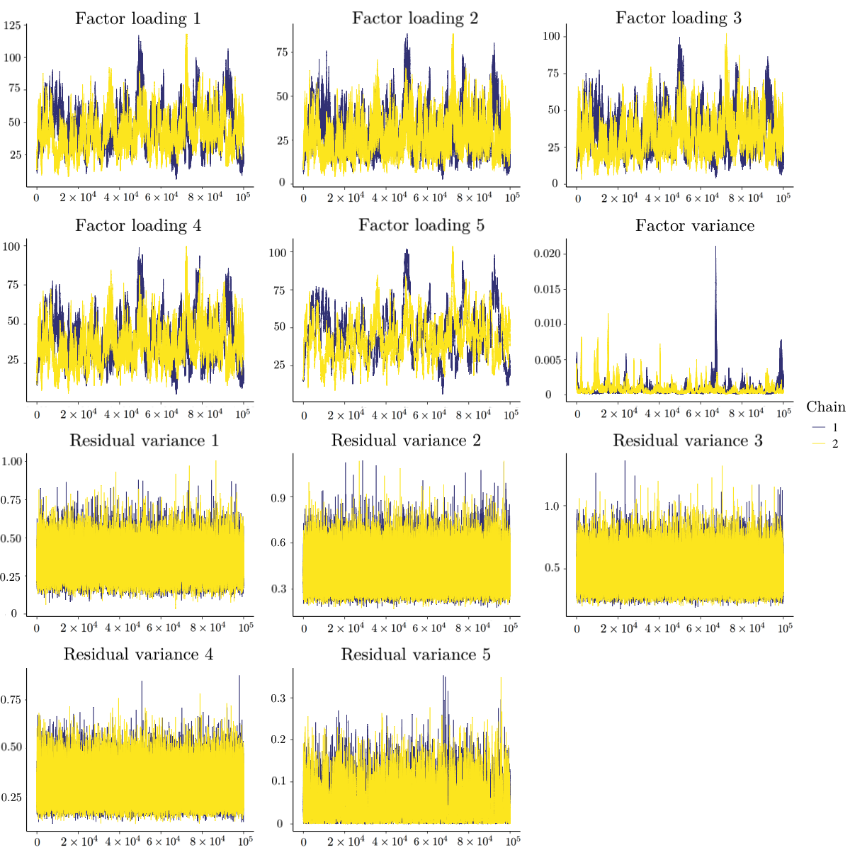
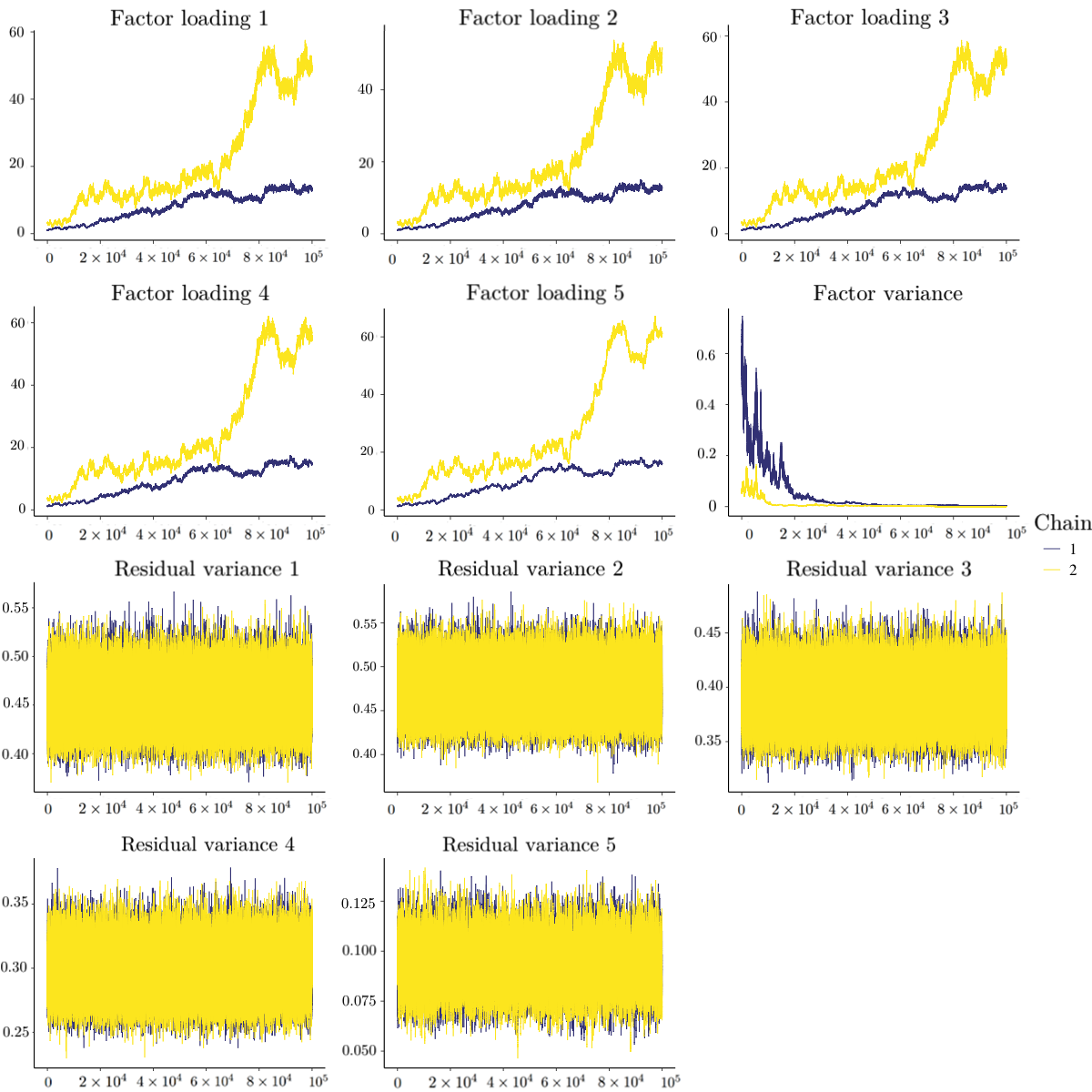
Besides quantitative diagnostic methods, the trace plot method could provide another piece of information. Figure 1 presents the trace plots of the 11 parameters when $N=50$ with $10^{5}$ iterations after the initial burn-in period. In this replication, different indices gave inconsistent conclusion: the upper bound of RSPF of the factor variance was 1.32, but the MRSPF was 1.07 and the absolute values of Geweke of all parameters were within 1.15. The trace plots for the factor variance and the 5th residual variance in Figure 1 showed several high peaks and were somewhat truncated at 0. This pattern is suspicious, which may be the signal of non-convergence, although MRSPF and Geweke’s diagnostic indicated convergence in this case. Thus, we suggest using both quantitative diagnostics and visual inspection in practice. When the sample size $N$ became large, the prior information could not bound the posterior distributions. As shown in Figure 2, when $N=1000$, the posterior samples of factor loadings kept going up and the two chains did not mix, and the posterior samples of factor variances were almost fixed at 0. In this case, the PSRFs (and their upper bounds) for factor loadings and factor variance and MPSRF were above 1.1, and the several absolute values of the Geweke’s diagnostic (especially for the factor loadings and factor variance) were larger than 1.96.
We summarize other conclusions as below. First, for $PSRF_{upper}>1.1$, $PSRF>1.1$, and $MPSRF>1.1$, more iterations made reaching convergence conclusions easier and thus increased the Type II error rates. More iterations increased the Type II error rates for $\left |Geweke\right |>1.96$ when $N$ was small. Second, because using PSRF is less conservative than using the upper bound, $PSRF>1.1$ had larger Type II error rates compared to $PSRF_{upper}>1.1$. $MPSRF>1.1$ also had larger Type II error rates than $PSRF_{upper}>1.1$. Third, with the positivity constraint, $\left |Geweke\right |>1.96$ had similar Type II error rates as $PSRF>1.1$.
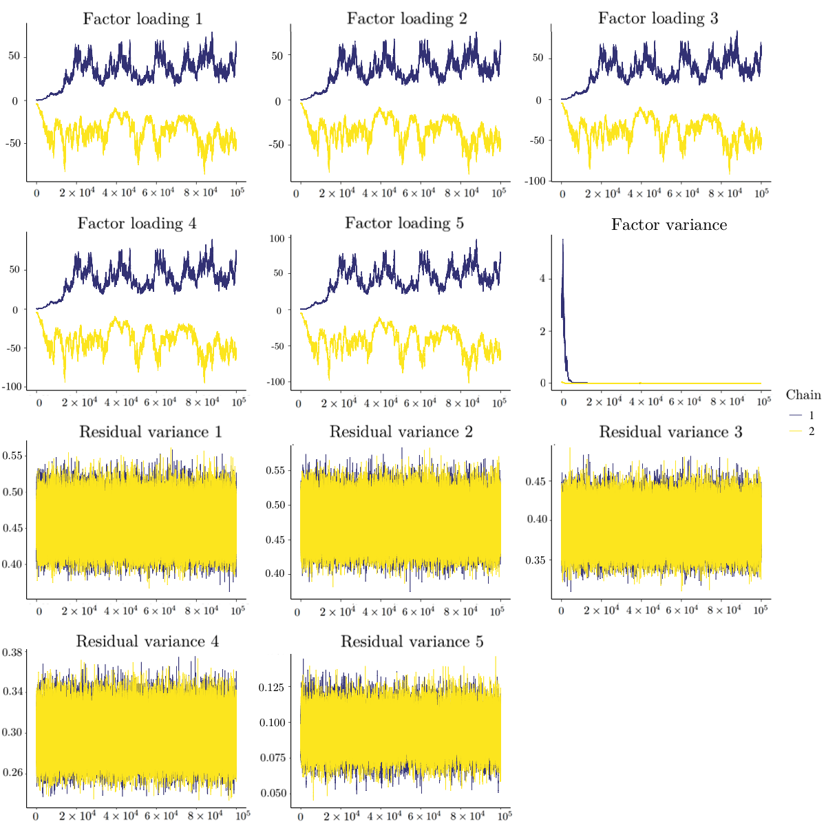
Now we move to the case without a positivity constraint on factor loadings where sign reflection invariance could cause non-convergence. We report the Type II error rates without a positivity constraint across 1000 replications of the four indices in Table 7. To better illustrate the posterior samples, Figure 3 presents the trace plots of the 11 parameters when $N=1000$ without a positivity constraint. The two chains of factor loadings did not mix well. PSRF and MPSRF can test whether multiple chains mix well, whereas Geweke’s test cannot test this feature of the posterior samples. As a consequence, the Type II error rates of $\left |Geweke\right |>1.96$ were much larger than $PSRF_{upper}>1.1$ , $PSRF>1.1$, and $MPSRF>1.1$, which was different from the positivity constraint case. Similar to the positivity constraint case, $PSRF>1.1$ and $MPSRF>1.1$ had larger Type II error rates than $PSRF_{upper}>1.1$.
| $PSRF_{upper}>1.1$ | ||||||||
| $N$ | $T$ | 250 | $5\times 10{}^{2}$ | $1.5\times 10{}^{3}$ | $2.5\times 10{}^{3}$ | $5\times 10{}^{3}$ | $2.5\times 10{}^{4}$ | $5\times 10^{4}$ |
| 50 | 0 | 0 | 0.002 | 0.044 | 0.043 | 0.165 | 0.207 | |
| 100 | 0 | 0 | 0.008 | 0.019 | 0.03 | 0.07 | 0.243 | |
| 200 | 0 | 0.002 | 0.004 | 0.013 | 0.073 | 0.163 | 0.243 | |
| 500 | 0 | 0 | 0 | 0.001 | 0.006 | 0.022 | 0.051 | |
| 1000 | 0 | 0 | 0 | 0.001 | 0.006 | 0.047 | 0.059 | |
| $PSRF>1.1$
| ||||||||
| $N$ | $T$ | 250 | $5\times 10{}^{2}$ | $1.5\times 10{}^{3}$ | $2.5\times 10{}^{3}$ | $5\times 10{}^{3}$ | $2.5\times 10{}^{4}$ | $5\times 10^{4}$ |
| 50 | 0.004 | 0 | 0.005 | 0.142 | 0.12 | 0.241 | 0.302 | |
| 100 | 0.006 | 0.002 | 0.038 | 0.05 | 0.11 | 0.182 | 0.371 | |
| 200 | 0 | 0.006 | 0.025 | 0.031 | 0.187 | 0.342 | 0.436 | |
| 500 | 0 | 0 | 0.003 | 0.004 | 0.015 | 0.056 | 0.104 | |
| 1000 | 0 | 0 | 0.001 | 0.001 | 0.021 | 0.115 | 0.125 | |
| $MPSRF>1.1$
| ||||||||
| $N$ | $T$ | 250 | $5\times 10{}^{2}$ | $1.5\times 10{}^{3}$ | $2.5\times 10{}^{3}$ | $5\times 10{}^{3}$ | $2.5\times 10{}^{4}$ | $5\times 10^{4}$ |
| 50 | 0.003 | 0.001 | 0.011 | 0.268 | 0.271 | 0.431 | 0.438 | |
| 100 | 0.009 | 0.002 | 0.05 | 0.112 | 0.206 | 0.478 | 0.54 | |
| 200 | 0.001 | 0.007 | 0.037 | 0.069 | 0.347 | 0.645 | 0.728 | |
| 500 | 0 | 0 | 0.003 | 0.006 | 0.031 | 0.109 | 0.21 | |
| 1000 | 0 | 0 | 0.001 | 0.003 | 0.028 | 0.261 | 0.276 | |
| $\left |Geweke\right |>1.96$
| ||||||||
| $N$ | $T$ | 250 | $5\times 10{}^{2}$ | $1.5\times 10{}^{3}$ | $2.5\times 10{}^{3}$ | $5\times 10{}^{3}$ | $2.5\times 10{}^{4}$ | $5\times 10^{4}$ |
| 50 | 0.28 | 0.022 | 0.159 | 0.176 | 0.14 | 0.76 | 0.698 | |
| 100 | 0.128 | 0.011 | 0.374 | 0.623 | 0.379 | 0.592 | 0.454 | |
| 200 | 0.037 | 0.193 | 0.018 | 0.281 | 0.303 | 0.402 | 0.836 | |
| 500 | 0.207 | 0.464 | 0.195 | 0.371 | 0.044 | 0.555 | 0.873 | |
| 1000 | 0.041 | 0.088 | 0.228 | 0.012 | 0.101 | 0.378 | 0.135 | |
Bayesian statistics has grown vastly and has been widely used in psychological studies in recent decades given the surge in computational power. Convergence assessment is critical to Markov chain Monte Carlo (MCMC) algorithms. Without appropriate convergence assessment, we cannot make reliable statistical inferences from the MCMC samples. Various quantitative diagnostic methods have been proposed for assessing convergence. The general recommendation is to use all the possible diagnostics because no method outperforms the others consistently. We endorse this recommendation if applying all diagnostic methods is feasible. However, there are situations where we cannot perform multiple convergence diagnostics. For example, in simulation studies, researchers rarely use multiple diagnostics to check convergence for all replications because it is time-consuming. Additionally, some software only provides one convergence diagnostic (e.g., BUGS and Mplus) and has created barriers for applied researchers to perform all convergence assessments. We do not object to the use of multiple or all convergence diagnostics simultaneously, but we would like to provide a guideline for applied researchers when resources are limited and it is not possible to perform multiple diagnostics. In the current paper, we focused on Gelman and Rubin’s diagnostic (PSRF), Brooks and Gleman’s multivariate diagnostic (MPSRF), and Geweke’s diagnostic.
Previous studies that reviewed and/or compared different convergence diagnostics using hypothetical examples did not study their statistical properties such as Type I error rates and Type II error rates (Brooks and Roberts, 1998; Cowles and Carlin, 1996; El Adlouni et al., 2006). In this study, we evaluated these two statistical properties of the seven diagnostic criteria via simulation studies. Based on the results of simulation studies, we obtained a better understanding of the answers to the three unsolved questions listed in the introduction section. For the first question, if we only can choose one diagnostic, which one should we used? We recommend the upper bound of PSRF for three reasons. First, in terms of the Type I error rates, the upper bound of PSRF and PSRF required fewer iterations to achieve an acceptable Type I error rate ($\leq 5\%$), compared to MPSRF the Geweke’s diagnostic (see Table 4). Second, in terms of the Type II error rates, PSRF led to higher Type II error rates than the upper bound of PSRF when the model was unidentified and the MCMC chains could not converge. $PSRF_{upper}>1.1$ had the smallest Type II error rates among $PSRF_{upper}>1.1$ , $PSRF>1.1$ , $MPSRF>1.1$, and $\left |Geweke\right |>1.96$. Overall, balancing both the Type I error rate and Type II error rate, we recommend using the upper bound of PSRF. Third, PSRF and its upper bound could detect non-convergence due to bad mixing (e.g., the sign reflection invariance case) whereas Geweke’s diagnostic could not. But we also need to note that PSRF is criticized for relying on over-dispersed starting values.
For the second question, when the number of estimated parameters is large, should we rely on the diagnostic per parameter (i.e., PSRF) or the multivariate diagnostic (i.e., MPSRF)? MPSRF yielded higher Type I and Type II error rates than PSRF and the upper bound of PSRF. Therefore, we still recommend the upper bound of PSRF over MPSRF.
For the third question, should we allow a small proportion of the parameters (e.g., 5%) to have significant convergence test results but still claim convergence as a whole? Comparing $PSRF_{upper,5\%}>1.1$ and $PSRF_{upper}>1.1$, the minimal number of iterations to control the analysis-wise Type I error rates below 5% did not differ dramatically. As the number of iterations increased, their Type I error rates were the same (0%). It is also difficult to define how small the proportion of the parameters should be in a widely acceptable way. In this paper, we used 5%, but one may would like to use 1% or 10%. Hence, we do not suggest allowing a small proportion of the parameters to have significant convergence diagnosis results but still claim convergence at the analysis level.
We echo the recommendation from previous studies, which advocate the use of all possible diagnostics when software and computational source are available. But when one has to choose one diagnostic, we recommend the upper bound of PSRF ($PSRF_{upper}>1.1$). Even with a large number of parameters, we think it is better not to allow a 5% Type I error rate within each analysis. Additionally, we suggest using both quantitative diagnostics and visual inspection (e.g., trace plot) because trace plots provide extra information. For example, in simulation studies, one can randomly select several replications to check the trace plots, combined with the convergence rates from quantitative diagnostics.
The simulation code is available at https://github.com/hduquant/Convergence-Diagnostics.git. Correspondence should be addressed to Han Du, Pritzker Hall, 502 Portola Plaza, Los Angeles, CA 90095. Email: hdu@psych.ucla.edu.
Brooks, S. P. and Gelman, A. (1998). General methods for monitoring convergence of iterative simulations. Journal of Computational and Graphical Statistics, 7(4):434–455.
Brooks, S. P. and Roberts, G. O. (1998). Convergence assessment techniques for markov chain monte carlo. Statistics and Computing, 8(4):319–335.
Carpenter, B., Gelman, A., Hoffman, M. D., Lee, D., Goodrich, B., Betancourt, M., Brubaker, M., Guo, J., Li, P., and Riddell, A. (2017). Stan: A probabilistic programming language. Journal of Statistical Software, 76(1).
Cowles, M. K. and Carlin, B. P. (1996). Markov chain monte carlo convergence diagnostics: a comparative review. Journal of the American Statistical Association, 91(434):883–904.
El Adlouni, S., Favre, A.-C., and Bobée, B. (2006). Comparison of methodologies to assess the convergence of markov chain monte carlo methods. Computational Statistics & Data Analysis, 50(10):2685–2701.
Erosheva, E. A. and Curtis, S. M. (2017). Dealing with reflection invariance in bayesian factor analysis. Psychometrika, 82(2):295–307.
Garren, S. T. and Smith, R. L. (2000). Estimating the second largest eigenvalue of a markov transition matrix. Bernoulli, pages 215–242.
Gelfand, A. E. and Smith, A. F. (1990). Sampling-based approaches to calculating marginal densities. Journal of the American Statistical Association, 85(410):398–409.
Gelman, A., Carlin, J. B., Stern, H. S., and Rubin, D. B. (2014). Bayesian data analysis, volume 2. Chapman & Hall, London.
Gelman, A. and Rubin, D. B. (1992). Inference from iterative simulation using multiple sequences. Statistical Science, pages 457–472.
Geweke, J. (1992). Evaluating the accuracy of sampling-based approaches to the calculation of posterior moments. In Bayesian Statistics, pages 169–193. University Press.
Gilks, W. R., Richardson, S., and Spiegelhalter, D. J. (1996). Introducing markov chain monte carlo. In Gilks, W. R., Richardson, S., and Spiegelhalter, D. J., editors, Markov chain Monte Carlo in practice, pages 339 – 357. Chapman & Hall, London.
Hastings, W. K. (1970). Monte carlo sampling methods using markov chains and their applications. Biometrika, 57(1):97–109.
Heidelberger, P. and Welch, P. D. (1983). Simulation run length control in the presence of an initial transient. Operations Research, 31(6):1109–1144.
Johnson, V. E. (1996). Studying convergence of markov chain monte carlo algorithms using coupled sample paths. Journal of the American Statistical Association, 91(433):154–166.
Lee, M. D. (2008). Three case studies in the bayesian analysis of cognitive models. Psychonomic Bulletin & Review, 15(1):1–15.
Liu, C., Liu, J., and Rubin, D. B. (1992). A variational control variable for assessing the convergence of the gibbs sampler. In Proceedings of the American Statistical Association, Statistical Computing Section, pages 74–78.
Lynch, S. M. (2007). Introduction to applied Bayesian statistics and estimation for social scientists. Springer Science & Business Media.
Marsman, M., Schonbrodt, F. D., Morey, R. D., Yao, Y., Gelman, A., and Wagenmakers, E.-J. (2017). A bayesian bird’s eye view of ‘Replications of important results in social psychology’. Royal Society open science, 4(1):160426.
Muthén, L. and Muthén, B. (1998–2017). Mplus User’s Guide. 8th edition. Los Angeles, CA: Author.
Plummer, M., Best, N., Cowles, K., and Vines, K. (2015). Package ’coda’. URL http://cran. r-project. org/web/packages/coda/coda. pdf, accessed January, 25:2015.
Raftery, A. and Lewis, S. (1991). How many iterations in the gibbs sampler?
Spiegelhalter, D. J., Thomas, A., Best, N. G., Gilks, W., and Lunn, D. (1996). Bugs: Bayesian inference using gibbs sampling. Version 0.5,(version ii) http://www. mrc-bsu. cam. ac. uk/bugs, 19.
Van de Schoot, R., Kaplan, D., Denissen, J., Asendorpf, J. B., Neyer, F. J., and Van Aken, M. A. (2014). A gentle introduction to bayesian analysis: Applications to developmental research. Child Development, 85(3):842–860.
Van de Schoot, R., Winter, S. D., Ryan, O., Zondervan-Zwijnenburg, M., and Depaoli, S. (2017). A systematic review of ”bayesian” articles in psychology: The last 25 years. Psychological Methods, 22(2):217.
Walker, L. J., Gustafson, P., and Frimer, J. A. (2007). The application of bayesian analysis to issues in developmental research. International Journal of Behavioral Development, 31(4):366–373.