Keywords: Latent class analysis · Mixture models · Bayesian analysis
Latent class analysis (LCA) is a powerful mixture model that can be used to group individuals into homogeneous classes, types, or categories based on the responses to a set of observed variables or items. An important usage of LCA is to develop typologies based on the characteristics of the identified classes. LCA has been applied in a variety of substantive fields, such as profiles of personality (Merz & Roesch, 2011), differential diagnosis among mental disorders (Cloitre, Garvert, Weiss, Carlson, & Bryant, 2014), and dietary patterns among older adults (Harrington, Dahly, Fitzgerald, Gilthorpe, & Perry, 2014). Overviews of LCA can be found in Collins and Lanza (2010) and Depaoli (2021). Related and more complex models are discussed in Hancock, Harring, and Macready (2019).
In this tutorial, readers will learn how to perform LCA and two of its extensions using Bayesian methods. Real and simulated examples are adopted for illustration. The platform that will be used is R with the JAGS program installed. The reminder of the tutorial includes the following main sections. In Section 2, we provide a more formal introduction to LCA, where the LCA for binary items will be described in particular. Three fundamental issues associated with LCA are covered in Section 3. In Section 4, a real dataset used for illustration will be briefly introduced. The conventional LCA process is introduced in Section 5, which is followed by its Bayesian counterpart in Section 6. Section 7 provides readers with two related extensions. Section 8 displays a guidance for wrapping up the LCA results. The tutorial ends with a brief discussion.
The LCA models are under the umbrella of finite mixture models (McLachlan & Peel, 2000), where observations are assumed to have arisen from one of the components, each being modeled by a density function from a parametric family (e.g., exponential). A $K$-component mixture density of a $J$-dimensional random vector $\boldsymbol {y}_i$ can be expressed as
where $w_k$ indicates the mixing proportion1 of the $k$-th component with $\sum _k w_k=1$, $\boldsymbol {\lambda }_k$ the vector of unknown parameters of the $k$-th component, and $f\left (\boldsymbol {y}_i ; \boldsymbol {\lambda }_k\right )$ the $k$-th component density. Also, we introduce a latent classification variable, $c_i$, to represent the $i$-th individual’s class membership, where $c_i$ takes on discrete values $1, ..., K$, so that $c_i = k$ indicates that the $i$-th observation belongs to the $k$-th class.
Although not realistic, there is one primary assumption, local independence, that needs to be met in the traditional LCA. This assumption implies that the items are independent of each other given latent class, meaning that latent class membership explains all of the shared variance among the items. The advantage of making the assumption is that it simplifies the component-level density function to a product of item-level probability densities as follows

With the estimates, the posterior probability that an individual belongs to class $k$ can be calculated using Bayes’ rule

Now, let’s consider an LCA for binary items. Suppose we observe $J$ dichotomous variables, each of which contains $\{0, 1\}$ possible outcomes, for individuals $i = 1, \ldots , N$. We denote as $w_1, \ldots , w_K$ the $K$ mixing proportions with $\sum _{k=1}^K w_k = 1$. Let $y_{ij}$ be the observed value of the $j$-th variable such that $y_{ij} = 1$ if individual $i$ endorses the $j$-th item, and $y_{ij} = 0$ otherwise. Let $\pi _{jk}$ denote the item response probability (IRP) representing how likely an individual in class $k$ endorses the $j$-th item. Then the probability that an individual $i$ in class $k$ produces a particular set of $J$ outcomes on the items, assuming local independence, is the product

Therefore, the overall likelihood function across the $K$ classes for $\boldsymbol {y}_{i}$ is the weighted sum

and the posterior classification probability can be written as

The basic idea of parameter estimation is to find the parameter estimates that maximize the log-likelihood function; i.e., find those that yield the greatest likelihood of having generated the observed data. Therefore, we are usually looking for the global maxima. However, finding the global maximum can be particularly challenging for a gradient ascent algorithm (e.g., EM) when the log-likelihood function of a LCA model is non-concave and has multiple local maxima.
To avoid arriving at a local maximum, it is always preferable to estimate the model a couple of times with different sets of random initial values. The solution that the majority of the sets converge to can then be considered the maximum likelihood solution (McLachlan & Peel, 2000). Many software packages, such as the poLCA R package, have implemented the use of multiple sets of random initial values.
It frequently occurs that one or more maximum likelihood (ML) estimates of LCA models lie on the boundary of the parameter space, i.e., the estimates are $0$ or $1$. This issue not only results in numerical problems in the computation of the variance-covariance matrix, but renders the provided confidence intervals and significance tests for the parameters meaningless. Nonetheless, boundary estimates can be readily avoided by imposing priors in Bayesian inference.
For a mixture model with $K$ components, there are $K$! possible permutations of the labels. Label switching refers to the phenomenon where the likelihood of a mixture model is invariant for any permutations of its component labels.
Let $\mathcal {P}_{K}$ be the set of $K!$ permutations of $\{1, \ldots , K\}$. If for some $\rho \in \mathcal {P}_{K}$, define $\boldsymbol {\theta }^\rho :=(w_{\rho (1)}, \ldots , w_{\rho (K)}, \boldsymbol {\lambda }_{\rho (1)}, \ldots , \boldsymbol {\lambda }_{\rho (K)})$, then for any $\rho , \nu \in \mathcal {P}_{K}$,

In frequentist mixture models, label switching arises when working with resampling methods (e.g., bootstrap) and simulation studies. Label switching is a well-known and fundamental issue in Bayesian mixture analysis as well. In Bayesian inference, if there is no prior information that distinguishes between the mixture components, and the prior distribution is the same for the permutations of $\boldsymbol {\theta }$, then the posterior distribution will be symmetric. When such information is available, we can use a prior that imposes a constraint that makes the components unique. However, such a prior might no longer be conjugate, and the Gibbs sampler could lose its simplicity. In addition, the fact that label switching occurs both within and between Markov chains further complicates label switching.
Fortunately, ample relabeling approaches are available for correcting the label switching problem in different scenarios. Approaches proposed for frequentist inference can be found in Yao (2015) and O’Hagan et al. (2019). For Bayesian inference, Papastamoulis (2016) provides ad-hoc procedures relabeling MCMC samples.
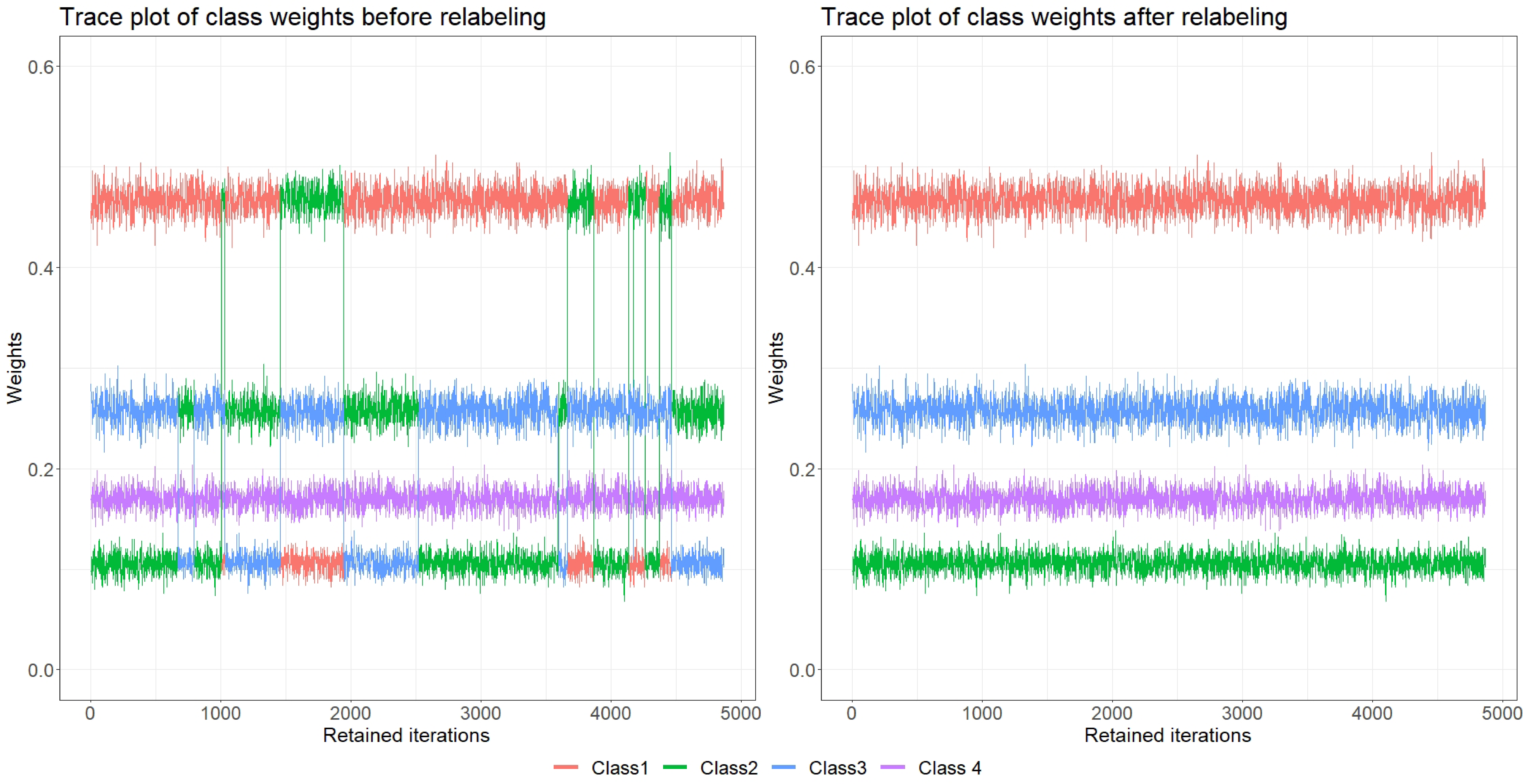
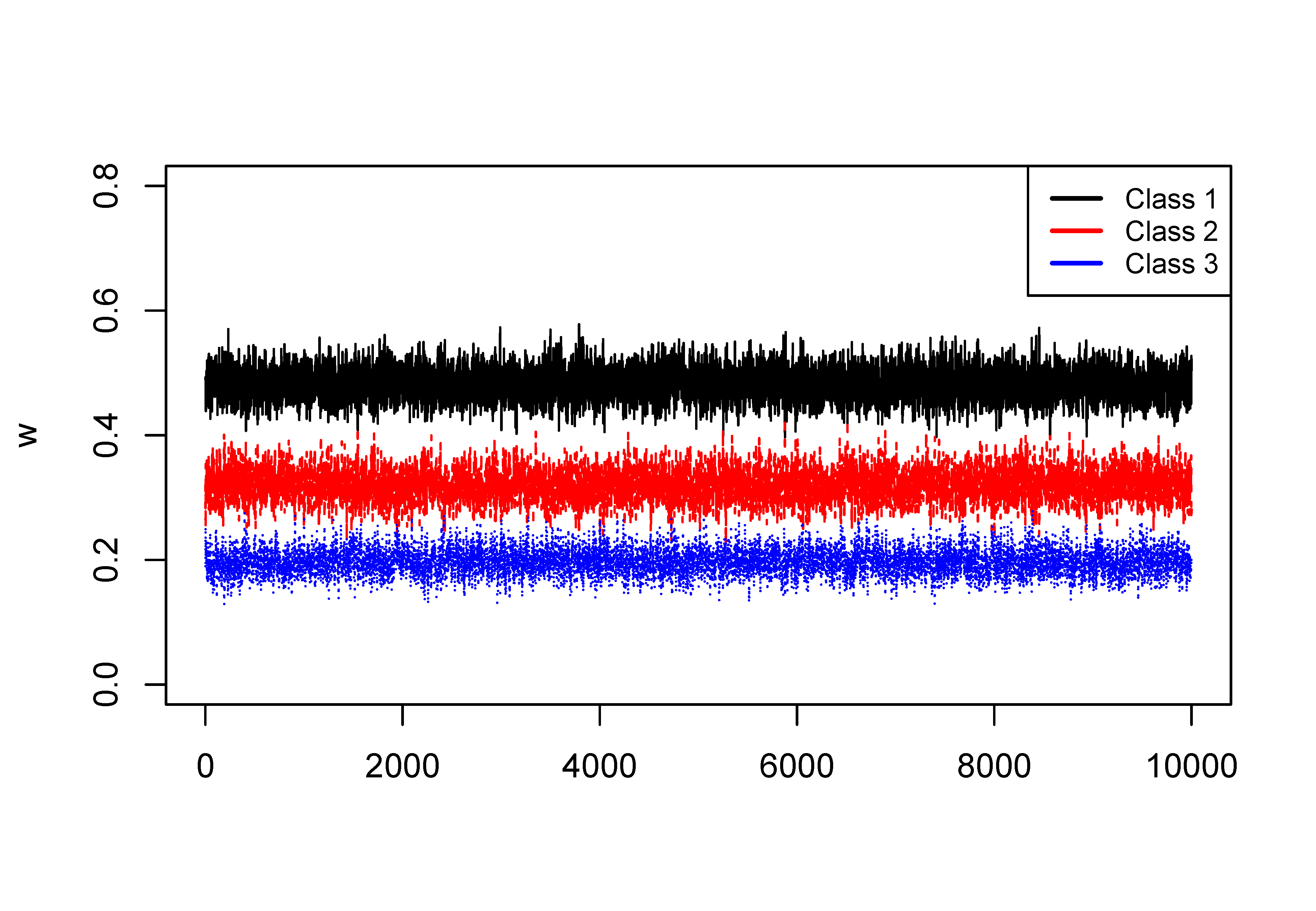
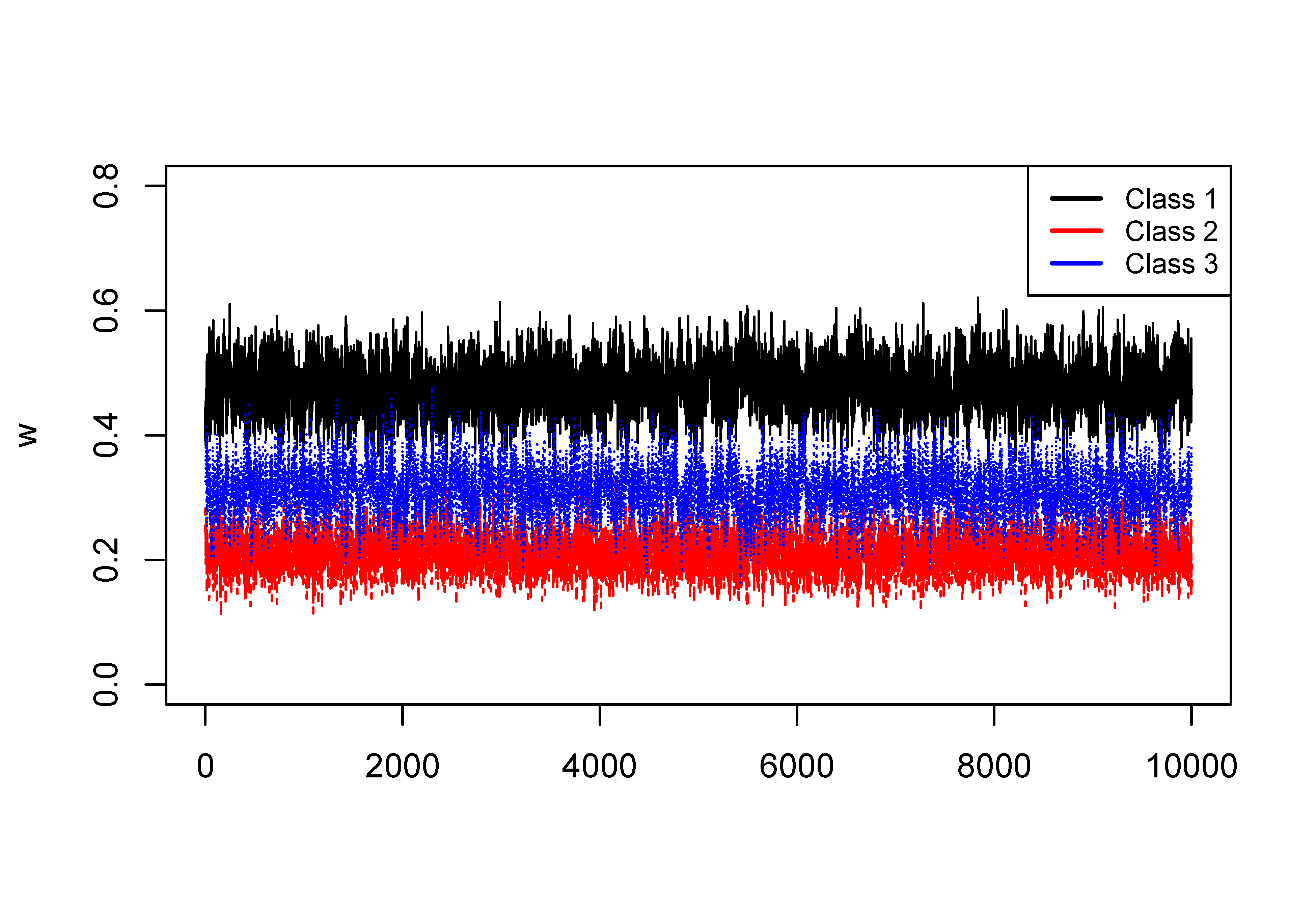
In the following example, we demonstrate the issue in a Markov chain. Plotted are MCMC traces for the class weights of a four-class solution using a simulated dataset. In the plot, one color indicates one parameter. The left-hand panel displays the trace plot of the class weights before relabeling, where signs of label switching are presented by the iterations drifted to different classes; whereas the right-hand panel represents the trace plot after relabeling, where no drifted iterations are found. Illustrative R code for solving label switching is available in the supplementary materials.
The National Youth Risk Behavior Survey (YRBS) is a school-based cross-sectional survey that has been conducted biennially by the Centers for Disease Control and Prevention (CDC) since 1991 to collect data on health habits and experiences among high school students across the United States.
To discover the unobserved types of health behaviors, we follow a previous study (Xiao, Romanelli, & Lindsey, 2019) and conduct an LCA on 13 health-behavior items in YRBS2019 that encompass four domains including: 1) diet (consumption of breakfast, fruits, juices, vegetables, milk, water, and soda), 2) physical activities (moderate and vigorous physical activity [MVPA], muscle-strengthening exercise [MSEs], and sports team participation [STP]), 3) sleeping time, and 4) media use (television [TV], computer/video games).
The items are dichotomized to $0$ and $1$, in which three items are reverse coded including television, computer/video games, and consumption of soda. A sample of 1,000 complete cases will be used for the analysis.
Determining the number of classes is always a challenging task in practice. The decision of how many classes to retain in LCA is conventionally made through the so-called class enumeration process. Class enumeration includes fitting a series of LCA models with increment of one in $K$ and selecting the “best” model via certain criterion (e.g., information criteria) or a set of criteria. To compare the criteria across the fittings, we often tabulate or plot the fit information for each model fitting, and study patterns to pick the optimal $K$. This process will be illustrated in Section 5.4. For a more detailed introduction to model fit and model selection in LCA, interested readers can refer to Section 4.3 of Collins and Lanza (2010).
A popular approach to summarizing uncertainty in posterior classification is entropy. In LCA, the entropy can be expressed as

where $\alpha _{ik}$ represents the posterior classification probability of individual $i$ defined as

A normalized version of $EN$, called relative entropy ($RE$), that scales $EN$ to the interval $[0,1]$ has been commonly used in LCA and is defined as

with $RE$ closer to 1 indicating less classification uncertainty and clearer assignment of individuals to latent classes. A $RE$ greater than $0.6$ is generally considered to be satisfactory class separation (Asparouhov & Muthen, 2014).
The last step of an LCA analysis is the interpretation of the retained solution, which involves more human judgement. The researchers need to examine the class-specific parameter estimates and then label each of the individual classes. Such labels should be related to the included items. It is beneficial to display the estimates in a plot (e.g., line plot). However, if a large number of classes is identified, it is more sensible to number the classes instead of assigning labels that cannot be easily distinguished verbally anymore. Another issue that may merit consideration is when the emergent classes differ merely quantitatively. In other words, the plotted lines are generally parallel. This phenomenon could indicate that a single sample was coerced into $K$ levels, such as low, medium, and high severity. When confronted with such classes, the solution should be interpreted cautiously.
LCA can be performed using a variety of commercial statistical packages, including Mplus (Muthen & Muthen, 1998-2017), SAS (SAS, 2016), STATA (STATA, 1985-2019), and Latent GOLD (Vermunt & Magidson, 2016). These commercial packages are user-friendly, can handle a wide range of mixture models, and offer cutting-edge approaches to handling missing data, covariates, and distal outcomes.
Various free R packages pertinent to mixture modeling are listed on the Cran Task Views: Psychometric Models and Methods and Clusters (https://cran.r-project.org/web/views), such as poLCA (Linzer & Lewis, 2011), MCLUST (Scrucca, Fop, Murphy, & Raftery, 2016), and tidyLPA (Rosenberg, Beymer, Anderson, van Lissa, & Schmidt, 2018). Haughton et al. (2009) provides a review of three packages, namely, Latent GOLD, MCLUST, and poLCA.
In this tutorial, we demonstrate the implementation of the frequentist LCA with poLCA, and the Bayesian LCA with JAGS.
The following chunk of code loads required packages for the entire tutorial.
library("poLCA")           # To use poLCA function
library("label.switching") # To address label switching
library("runjags")         # To use JAGS via R
library("glue")            # To insert R code within strings
library("gt")              # For pretty tables
library("knitr")           # To use the "kable" function
library("kableExtra")      # For more about kable
library("cowplot")         # For pretty plots
library("scatterplot3d")   # For 3-D plot
library("ggpubr")          # To use the "ggarrange" function
library("coda")            # To use Geweke’s diagnostic test
library("MASS")            # To use the "mvrnorm" function
library("tidyverse")       # For everything else...
This chunk of code loads saved datasets and outputs for the following sections to reduce knitting time.
load("C:/Users/Chris/Desktop/LCA/objects.RData")
To use the poLCA() function, the items must be coded as integer values starting at one for the first outcome category, and increasing to the maximum number of outcomes for each variable. Consequently, we add one to all the responses resulting in binary outcomes of $\{1, 2\}$.
dat <- dat.yrbs + 1 # poLCA only allows positive integers
Notice that a specific R function lca_re() is created for computing relative entropy. The reason is that poLCA defines entropy as a measure of dispersion (or concentration) in a probability mass function, which is different from the widely used definition (e.g., in Mplus). For computational details, readers can refer to the help document of poLCA.entropy() function.
# Function for computing relative entropy
lca_re <- function(x) {
  nom <- (sum(-x$posterior*log(x$posterior)))
  denom <- (nrow(x$posterior)*log(ncol(x$posterior)))
  re <- 1 - (nom/denom)
  if (is.nan(re) == TRUE) re <- NA
  return(re)
}
To specify an LCA model, poLCA() requires users to provide a model formula. For the basic LCA model without covariates, the formula takes the following form:
f <- cbind(Y1, Y2, Y3, Y4, Y5, Y6, Y7, Y8, Y9, Y10, Y11, Y12, Y13)
              ~ 1
where the observed variables or items are bound together within cbind(Y1, Y2, Y3, ...), and the 1 indicates the LCA model without covariates. For LCA with covariates, one must substitute the 1 with a function of covariates as follows:
f <- cbind(Y1, Y2, Y3, Y4, Y5, Y6, Y7, Y8, Y9, Y10, Y11, Y12, Y13)
              ~ X1 + X2 + X3
When there are a large amount of items, as in our example, we can define the formula with the following code to save line space and typing time:
J <- ncol(dat) # number of items
f <- as.formula(paste("cbind(",paste(paste0("Y",1:J),collapse=","),
")","~1"))
# This is equivalent to: f <- cbind(Y1,Y2,Y3,Y4,Y5,Y6,Y7,Y8,Y9,Y10,
#                                      Y11,Y12,Y13) ~ 1
To estimate the desired LCA model via the poLCA() function, users need to pass the model formula, the dataset stored as a data frame, and the number of classes to the formula, data, and nclass arguments, respectively. Information about the remaining optional arguments of the function can be obtained by entering the command help(poLCA) or simply ?poLCA at the R console window. Nevertheless, we would like to place an emphasis on the nrep argument, which specifies the number of times to estimate the model using different sets of random starting values. As discussed in Section 3.1, this is desirable to prevent solutions from converging to local instead of global maxima of the likelihood function. For example, we set nrep to $20$ in the following code. Complex models often require more replications, especially in high-stakes applications.
In addition, it should be noted that poLCA() only provides two fit indices, AIC and BIC, by default. Other fit indices (e.g., aBIC) can be calculated manually based on the model results as shown in the code below.
# Class enumeration from K=1 to K=6
out_lca <- list()   # container of model fittings
npar <- ll <- bic <- abic <- caic <- awe <- re <- c() # containers
        # of other information
set.seed(123)
for(k in 1:6){
  fit <- poLCA(formula=f, data=dat, nclass=k, maxiter=10000,
               tol=1e-5, nrep=20, verbose=F, calc.se=T)
  out_lca[[k]] <- fit
  npar[k] <- fit$npar
  ll[k]   <- fit$llik
  bic[k]  <- fit$bic
  abic[k] <- -2*(fit$llik) + fit$npar*log((fit$Nobs+2)/24)
  caic[k] <- -2*(fit$llik) + fit$npar*(log(fit$Nobs)+1)
  awe[k]  <- -2*(fit$llik) + 2*(fit$npar)*(log(fit$Nobs)+1.5)
  re[k]   <- round(lca_re(fit), 3)
}
class <- paste0("Class-", 1:6)

# Store information in a data frame
poLCA.tab <- data.frame("Class"=class, "Npar"=npar, "LL"=ll,
    "BIC"=bic, "aBIC"=abic, "CAIC"=caic, "AWE"=awe, "RE"=re)
See Table 1 for the summary of fit.
| Class | Npar | LL | BIC | aBIC | CAIC | AWE | RE |
| Class-1 | 13 | -7575.656 | 15241.11 | 15199.82 | 15254.11 | 15369.91 | NA |
| Class-2 | 27 | -7278.148 | 14742.81 | 14657.05 | 14769.81 | 15010.31 | 0.666 |
| Class-3 | 41 | -7171.830 | 14626.88 | 14496.66 | 14667.88 | 15033.10 | 0.721 |
| Class-4 | 55 | -7103.205 | 14586.34 | 14411.65 | 14641.34 | 15131.26 | 0.748 |
| Class-5 | 69 | -7075.080 | 14626.79 | 14407.65 | 14695.79 | 15310.43 | 0.764 |
| Class-6 | 83 | -7050.491 | 14674.33 | 14410.71 | 14757.33 | 15496.67 | 0.704 |
1 Npar = number of parameters;
| |||||||
2 LL = log data likelihood;
| |||||||
3 BIC = bayesian information criterion;
| |||||||
4 aBIC = sample size adjusted BIC;
| |||||||
5 CAIC = consistent Akaike information criterion;
| |||||||
6 AWE = approximate weight of evidence criterion;
| |||||||
7 RE = relative entropy.
| |||||||
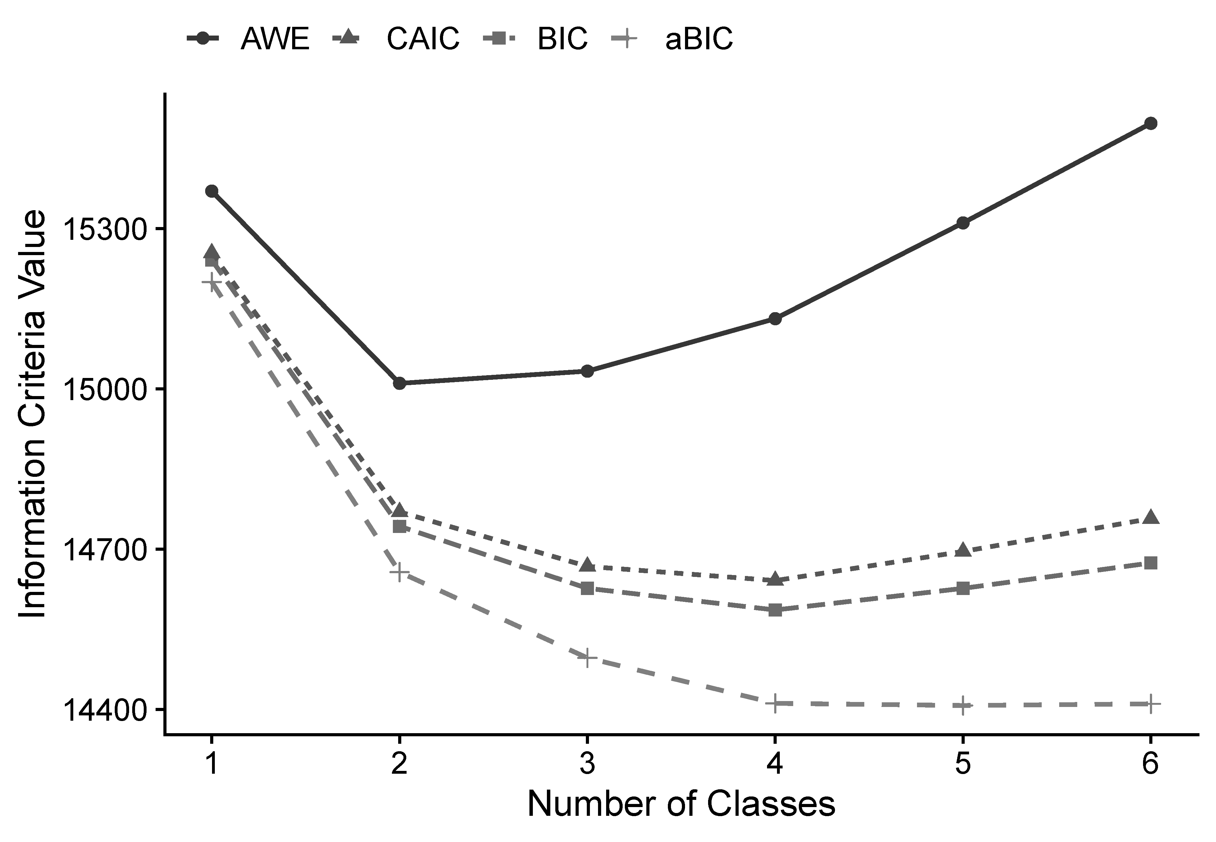
It is useful to plot the values of the selected information criteria (ICs) for visual inspection. Lower IC values signify a more optimal balance of model fit and parsimony. Ideally, a minimum value in the set of fittings indicates the optimal solution. However, it is not uncommon in practice that ICs continue to decrease as $K$ increases. That is, there is no global minimum. In such instances, the $K$ at an “elbow” of point of “diminishing returns” in model fit indices should be selected as the best solution. For the empirical example, the following elbow plot in Figure 2 suggests that the 2-class solution fits best based on AWE, whereas the 4-class solution is supported by CAIC, BIC, and aBIC. Therefore, the 4-class solution appears to be an appealing candidate. Next, this solution’s relative entropy is 0.748 (see Table 1), which is relatively high ($>0.6$) and indicative of satisfactory classification quality. Considering the current information, we decide on the 4-class solution.
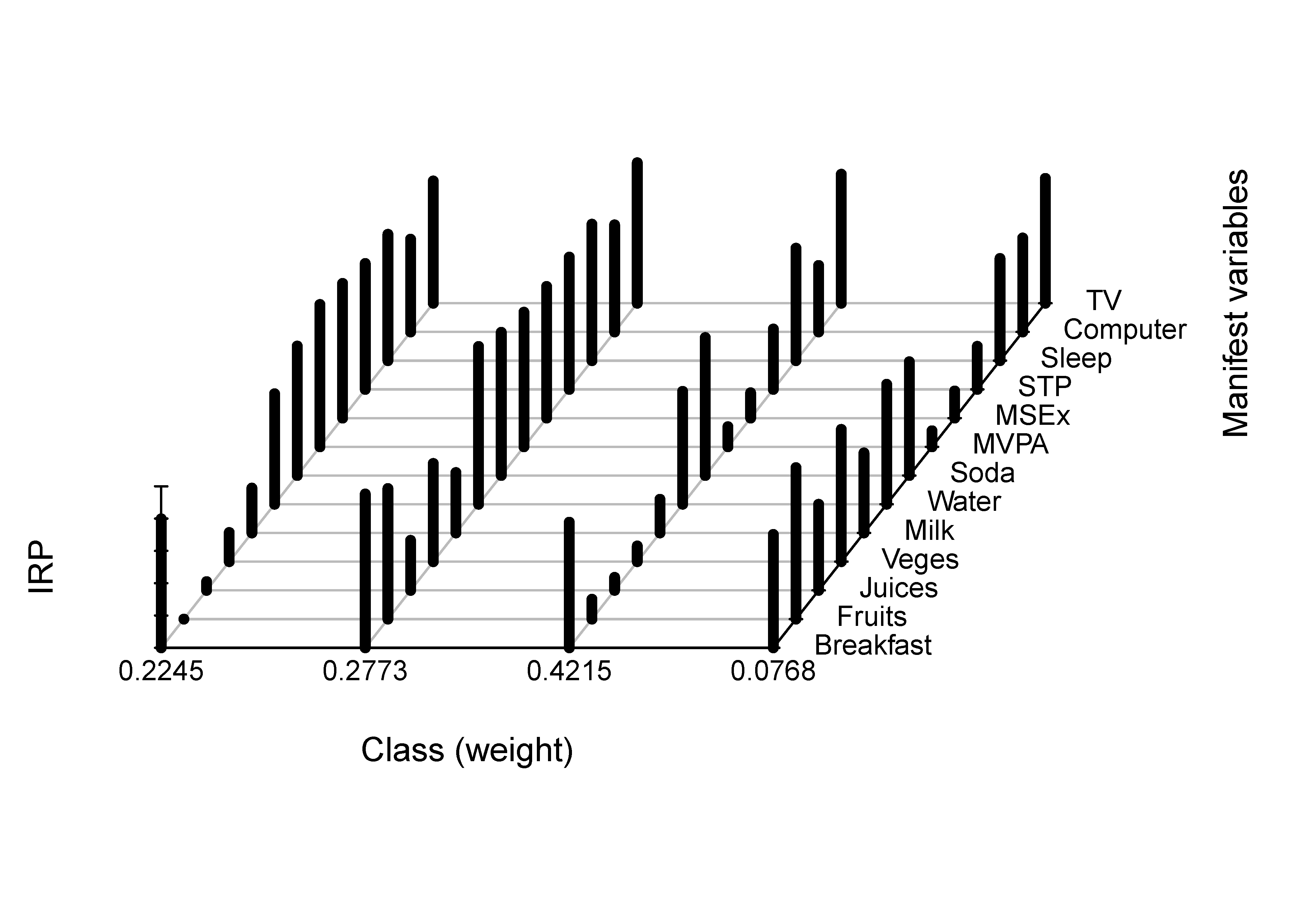
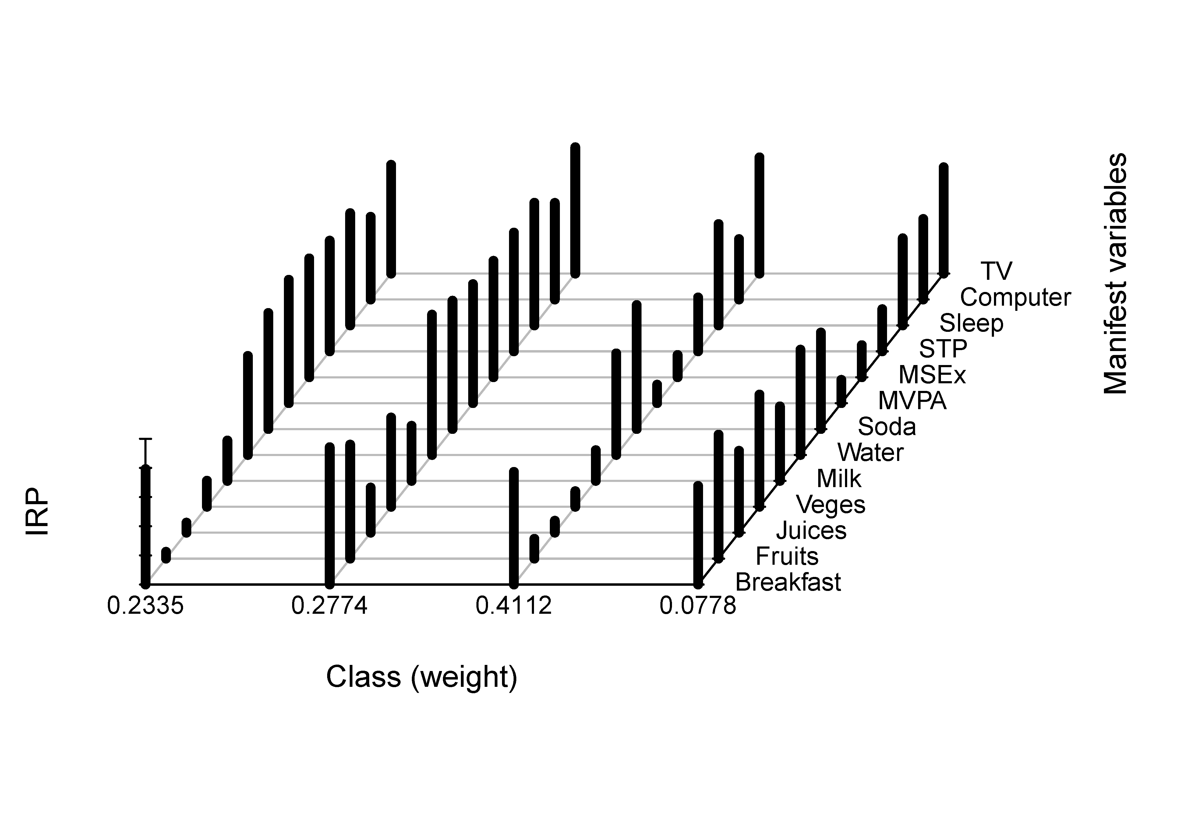
The profiles of the latent classes are shown in Figure 3.
According to the above item response probability plot, we can assign labels to the emergent classes. The first class is of medium size ($22.44\%$), and shows low engagement in health diet behavior, high engagement in exercise, and moderately high engagement in computer use. Hence, it can be characterized as the class of irregular diet, high exercise, moderately high computer use. The second class is small ($7.67\%$), and characterized by the highest engagement in healthy diet behaviors, low engagement in exercise, and relatively low computer use. We call this class the healthy diet, low exercise, relatively low computer use. The third class is the largest ($42.16\%$), and can be called the lowest engagement in health-promoting behaviors due to the low engagement in healthy diet behaviors and physical activities and the highest engagement in computer use. The fourth class, consistent engagement in health-promoting behaviors, is of medium size ($27.73\%$) and demonstrates moderate probabilities of a healthy dietary pattern, frequently physical activities, high probability of longer sleeping time, and low probability of playing computer more than 3 hours per day.
The model parameters of particular interest in LCA with binary items include mixing proportions $\boldsymbol {w}$ and binary IRPs $\boldsymbol {\pi }$. Here, $\boldsymbol {w}$ is assumed to follow a Dirichlet distribution denoted as

with the hyperparameters $d_1, \ldots , d_K$ which represent the prior proportion of individuals in each of the $K$ classes. The conjugate prior for IRP is the Beta distribution denoted as

where the hyperparameters $\alpha $ and $\beta $ represents the prior sample sizes for the number of individuals answering “Yes” and “No”, respectively.
The convergence diagnostic method adopted in this tutorial is Geweke’s test, which compares the location of the sampled parameter on two different time intervals of the chain. If the mean values of the parameter in the two time intervals are close to each other we then assume that the two parts of the chain have similar locations in the state space, and it is assumed that the two parts come from the same distribution. An absolute value of the $z$-score produced by Geweke’s test above $2$ could be considered as potentially problematic.
The following code specifies a JAGS model and stores the model in an R object called lca_bin. In fact, the model can be specified as a character string within R, or in an external text file. The former avoids the need for multiple text files, whereas the latter is preferred for more complex model formulations. In the tutorial, we adopt the former way.
Every model specification must begin with informing JAGS that it is a model specification using the model{} block. Within the model block, we specify data likelihood for every single data point using a for loop. Note that, there are two types of data in a mixture model$-$unobserved class membership $\boldsymbol {z}$ and observed data $\boldsymbol {y}$. Thus, we specify likelihood for $\boldsymbol {z}$ and $\boldsymbol {y}$, respectively, as shown in the “likelihood specification” chunk. First, we let $z[i]$ follows a categorical distribution with the dcat() call where $w[1:K]$ is a vector of non-negative mixing proportions of length $K$. Second, the likelihood for $\boldsymbol {y}$ is specified through a nested for loop because there are two indices (i.e., $i=1,\ldots ,N$ and $j=1,\ldots ,J$) associated with each data point of $\boldsymbol {y}$, and we let $y[i,j]$ follow a Bernoulli distribution with the dbern() call where $\pi [j,z[i]]$ represents the IRP for the $j$-th item within the $z[i]$-th class.
After specifying the data likelihood, we then impose priors on the model parameters (see the “prior specification” chunk). As discussed in Section 6.1, we impose Dirichlet and beta priors on mixing proportions ($\boldsymbol {w}$) and IRPs ($\boldsymbol {\pi }$), respectively.
# Build model: LCA for binary items
lca_bin <- "
model{
      #===========================
      # likelihood specification
      #===========================

      for(i in 1:N) {
        Z[i] ~ dcat(w[1:K]) # class membership for the i-th subject
        for(j in 1:J) {
          Y[i,j] ~ dbern(pi[j,Z[i]]) # Bernoulli density function
        }
      }

      #===========================
      # prior specification
      #===========================

      # --------- w ---------
      w[1:K] ~ ddirch(alpha[1:K])   # Dirichlet prior for
                                    # mixing proportions
      for(k in 1:K) {alpha[k] <- 1}

      # --------- pi ---------
      for(k in 1:K) {
        for(j in 1:J) {
          pi[j,k] ~ dbeta(3,3)      # beta prior for conditional
                                    # probabilities
        }
      }
}"
Users of JAGS have the option of supplying their own initial values or just using those generated by the random number generators (RNGs). For user-specified initial values, list starting values for each of the parameters in the model as follows:
# User-specified initial values
inits <- list(list(w=rep(0.25,4), pi=matrix(rbeta(J*K.est,3,3),
              nrow=J, ncol=K.est)))
There are four RNGs provided by the base module in JAGS with the following names:
“base::Wichmann-Hill”
“base::Marsaglia-Multicarry”
“base::Super-Duper”
“base::Mersenne-Twister”
To set the starting state of the RNG, one can simply supply the name of the RNG and its seed (e.g., 111) as shown in the following code:
# Automatically generated initial values
inits <- list(".RNG.name"="base::Wichmann-Hill", ".RNG.seed"=111)
We need to bundle the data and constants used in the JAGS model into a list that JAGS can read (see the Dat object in the following code). The call to run.jags() reads, complies, executes, and returns the model information along with MCMC samples and summary statistics. Before a model can be executed, the run.jags() function requires a valid JAGS model to be passed to the model argument and a character string of monitored parameters to the monitor argument.
Furthermore, the function allows users to specify additional arguments, including but not limited to: 1) the method with which to call JAGS (e.g., rjags); 2) number of Markov chains to run (e.g., n.chain=1); 3) the number of adaptive iterations used at the start of the chain (e.g., adapt=1000); 4) the number of burnin iterations (e.g., burnin=1000); 5) number of iterations per chain (e.g., sample=10000) in addition to the adaptive and burnin iterations; and 6) thinning interval for monitors (e.g., thin=1).
# Bundle data for JAGS
Dat <- list("Y"=as.matrix(dat.yrbs), "N"=N, "J"=J, "K"=4)
# Run the analysis
set.seed(1234)
out_bin <- run.jags(model=lca_bin, monitor=c(’w’,’pi’),
                    data=Dat, inits=inits, method="rjags",
                    n.chains=1, adapt=1000, burnin=1000,
                    sample=10000, thin=1)
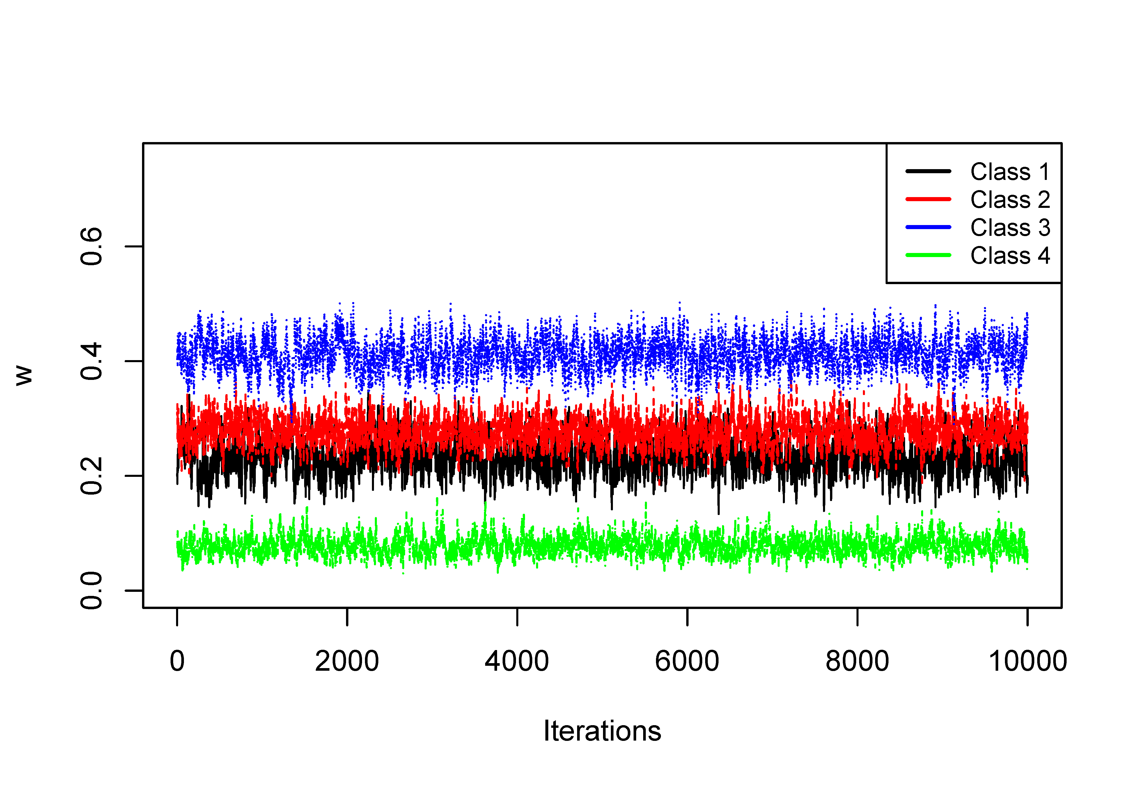
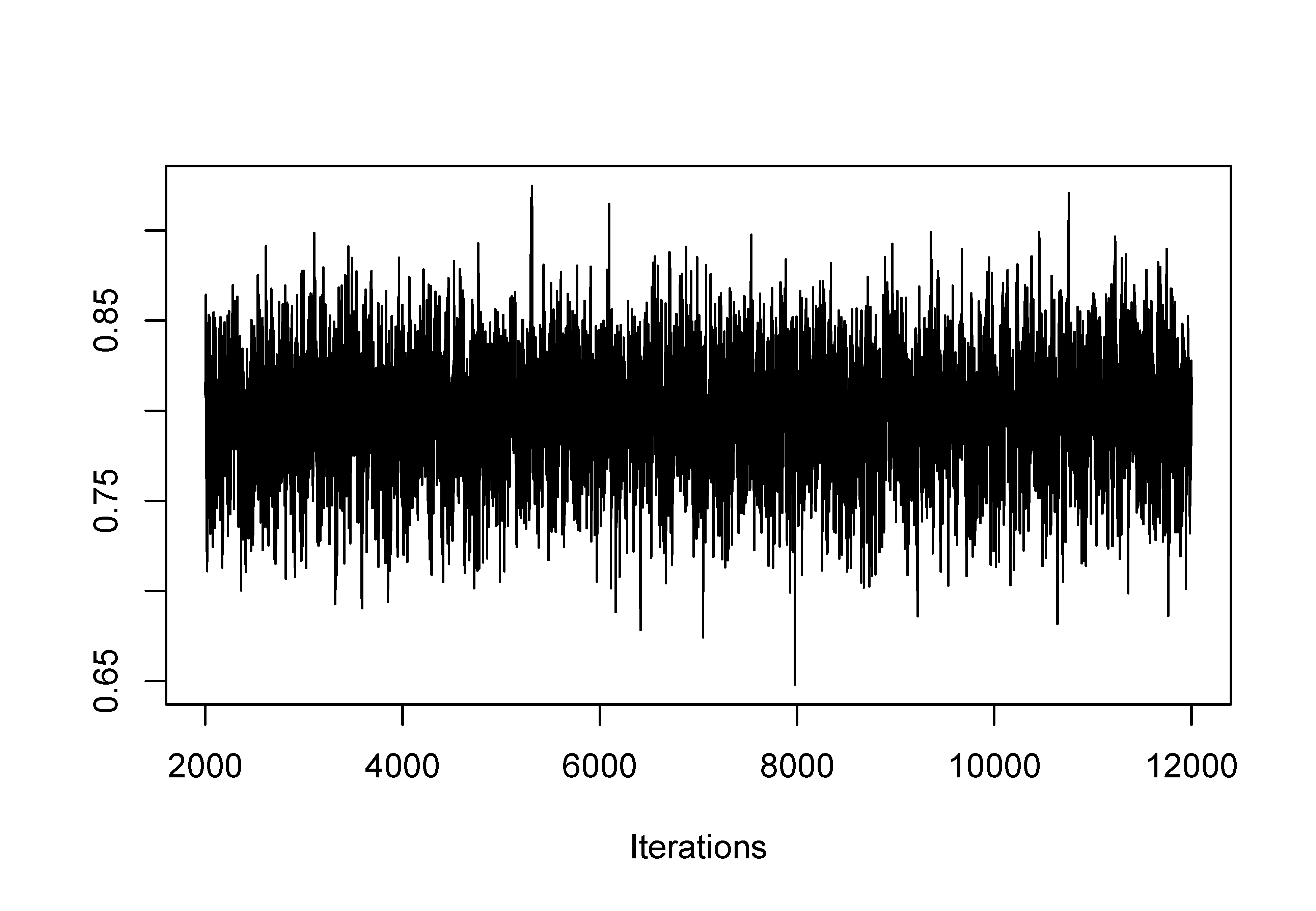
The trace plots of the weight of each class are displayed in Figure 4 and from it, no signs of label switching are found.
Note that the start argument of the window() function include the adaption (i.e., na) and burn-in (i.e., nb) phases, so if one has 12,000 iterations with 1,000 adaption and 1,000 burn-in samples, the following code will retain the iterations from 2,001 to 12,000.
na <- 1000; nb <- 1000
out.burn <- window(out_bin$mcmc, start=na+nb+1)
con.diag <- geweke.diag(out.burn)
# |z| > 2 is potentially problematic
flag.cov <- which(abs(con.diag[[1]]$z)>2)
# double check via trace plot
traceplot(out.burn[[1]][ ,flag.cov])
sum.stats <- summary(out.burn)         # summary statistics
post.means <- sum.stats$statistics[,1] # posterior means

# Note: pi[j,k] is the IRP of the j-th item in the k-th class
round(post.means, digits=3)
##     w[1]     w[2]     w[3]     w[4]  pi[1,1]  pi[2,1]  pi[3,1]  pi[4,1]
##    0.234    0.277    0.411    0.078    0.792    0.047    0.069    0.179
##  pi[5,1]  pi[6,1]  pi[7,1]  pi[8,1]  pi[9,1] pi[10,1] pi[11,1] pi[12,1]
##    0.277    0.680    0.797    0.847    0.816    0.760    0.770    0.568
## pi[13,1]  pi[1,2]  pi[2,2]  pi[3,2]  pi[4,2]  pi[5,2]  pi[6,2]  pi[7,2]
##    0.747    0.943    0.783    0.310    0.613    0.378    0.963    0.881
##  pi[8,2]  pi[9,2] pi[10,2] pi[11,2] pi[12,2] pi[13,2]  pi[1,3]  pi[2,3]
##    0.817    0.799    0.815    0.842    0.663    0.867    0.773    0.136
##  pi[3,3]  pi[4,3]  pi[5,3]  pi[6,3]  pi[7,3]  pi[8,3]  pi[9,3] pi[10,3]
##    0.083    0.107    0.211    0.697    0.851    0.127    0.153    0.370
## pi[11,3] pi[12,3] pi[13,3]  pi[1,4]  pi[2,4]  pi[3,4]  pi[4,4]  pi[5,4]
##    0.696    0.415    0.798    0.677    0.851    0.562    0.770    0.512
##  pi[6,4]  pi[7,4]  pi[8,4]  pi[9,4] pi[10,4] pi[11,4] pi[12,4] pi[13,4]
##    0.723    0.663    0.160    0.220    0.289    0.598    0.553    0.730
Compared with Figure 3, the class profiles yielded by the Bayesian LCA (Figure 6) look quite similar to that provided by the conventional LCA.
This section focuses on MMLCA for which observed variables are a mix of binary and continuous data. Suppose we observe $M$ variables consisting of $J$ binary variables and $L$ continuous variables for individuals $i=1, \cdots , N$. Let $u_{ij}$ be the observed value of the $j$-th binary item such that $u_{ij}=1$ if the $i$-th individual endorses the item (i.e., answer “Yes”), and $u_{ij}=0$ otherwise, where $j=1, \ldots , J$; let $v_{il}$ be the observed value of the $l$-th continuous item.
Assuming local independence, the probability that an individual $i$ in class $k$ produces a particular set of $M=J+L$ responses $y_i=\{u_{i1},u_{i2},\ldots ,u_{iJ}; v_{i1},v_{i2},\ldots ,v_{iL}\}$ is a finite mixture of conditional densities

where $g\left (\boldsymbol {u}_i \mid k\right )$ is the conditional density of the vector of observed binary items and $g\left (\boldsymbol {v}_i \mid k\right )$ is the conditional density of the vector of observed continuous items for the $i$-th individual given the $k$-th class, respectively.
Because of the local independence assumption, the two conditional densities can be further expanded. The $g\left (\boldsymbol {u}_i \mid k\right )$ can be expressed as a product of Bernoullis

where $\pi _{jk}$ represents the class-specific item response probability (IRP) that observations in the $k$-th class endorse the $j$-th binary variable; the $g\left (\boldsymbol {v}_i \mid k\right )$ can be written as a product of univariate Gaussians

where $\mu _{lk}$ and $\sigma _{lk}$ represent the mean and standard deviation of the $l$-th continuous variable, respectively.
Following the priors in LCA for binary items, we specify Dirichlet prior and Beta prior to mixing proportions and IRPs, respectively

For the parameters associated with the continuous items, we specify normal prior and Gamma prior to mean and precision ($\tau = 1/\sigma ^2$), respectively

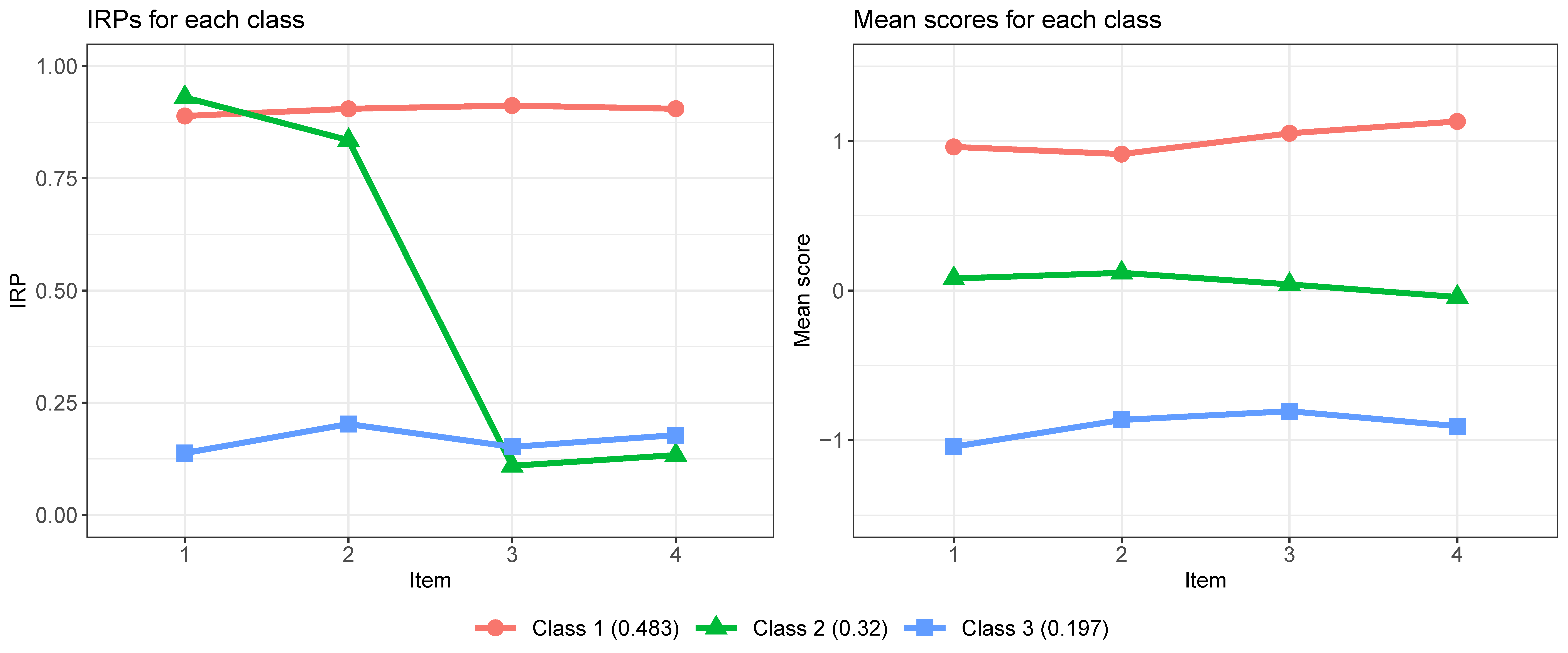
We simulate a dataset of 500 subjects from an MMLCA model with 3 classes and 8 items (4 binary and 4 continuous). The parameters shown in Table 2 serve as the population values for the data generating model. Each subject’s class membership is generated from unequal class sizes ($\boldsymbol {w}$) of 0.5, 0.3, and 0.2. For the binary items, the class-specific response probabilities ($\boldsymbol {\pi }$) are set to 0.9 in Class 1, to 0.9 for the first half of the items and 0.1 to the other half in Class 2, and to 0.1 in Class 3. For the continuous items, the class-specific item means ($\boldsymbol {\mu }$) are set to 1 in class 1, to 0 in Class 2, and to $-1$ in Class 3, with the item variances ($\boldsymbol {\sigma }^2$) fixed at 1 over the three classes.
| Class | w | $\pi $ | $\mu $ | $\sigma ^2$ |
| 1 | 0.5 | 0.9, 0.9, 0.9, 0.9 | 1, 1, 1, 1 | 1, 1, 1, 1 |
| 2 | 0.3 | 0.9, 0.9, 0.1, 0.1 | 0, 0, 0, 0 | 1, 1, 1, 1 |
| 3 | 0.2 | 0.1, 0.1, 0.1, 0.1 | -1, -1, -1, -1 | 1, 1, 1, 1 |
# Build model: LCA for binary and continuous items
lca_mix <- "
model{
      #===========================
      # likelihood specification
      #===========================

      for(i in 1:N) {
        Z[i] ~ dcat(w[1:K]) # Class membership for the i-th subject
        for(j in 1:J) {
          Y[i,j] ~ dbern(pi[j,Z[i]]) # Bernoulli density function
        }
        for(l in 1:L) {
          X[i,l] ~ dnorm(mu[l,Z[i]], tau[l,Z[i]]) # normal density
        }
      }

      #===========================
      # prior specification
      #===========================

      # --------- w ---------
      w[1:K] ~ ddirch(alpha[1:K])      # Dirichlet prior for
                                       #mixing proportions
      for(k in 1:K) {alpha[k] <- 1}

      # --------- pi ---------
      for(k in 1:K) {
        for(j in 1:J) {
          pi[j,k] ~ dbeta(3,3)         # beta prior for IRPs
        }
      }

      # --------- mu & tau ---------
      for(k in 1:K) {
        for(l in 1:L) {
          mu[l,k] ~ dnorm(0,1.0E-6)    # normal prior for mean
          tau[l,k] ~ dgamma(0.01,0.01) # gamma prior for precision
        }
      }
}"
# Automatically generated initial values
inits <- list(list(".RNG.name"="base::Wichmann-Hill",
        ".RNG.seed"=111))
# Bundle data for JAGS
Dat <- list("Y"=dat.mmlca[,1:J], "X"=dat.mmlca[,(J+1):(J+L)],
            "N"=N, "J"=J, "L"=L, "K"=3)

# Run the analysis
set.seed(1234)
out_mix <- run.jags(model=lca_mix, monitor=c(’w’,’pi’,’mu’,’tau’),
              data=Dat, inits=inits, method="rjags", n.chains=1,
              adapt=1000, burnin=1000, sample=10000, thin=1)
Similarly, no signs of label switching are found in Figure 7.
na <- 1000; nb <- 1000
out.burn <- window(out_mix$mcmc, start=na+nb+1)
con.diag <- geweke.diag(out.burn)
flag.noncov <- which(abs(con.diag[[1]]$z)>2)
sum.stats <- summary(out.burn)         # summary statistics
post.means <- sum.stats$statistics[,1] # posterior means
round(post.means, digits=3)
##     w[1]     w[2]     w[3]  pi[1,1]  pi[2,1]  pi[3,1]  pi[4,1]  pi[1,2]
##    0.483    0.320    0.197    0.889    0.905    0.912    0.905    0.930
##  pi[2,2]  pi[3,2]  pi[4,2]  pi[1,3]  pi[2,3]  pi[3,3]  pi[4,3]  mu[1,1]
##    0.835    0.109    0.133    0.138    0.203    0.152    0.178    0.960
##  mu[2,1]  mu[3,1]  mu[4,1]  mu[1,2]  mu[2,2]  mu[3,2]  mu[4,2]  mu[1,3]
##    0.912    1.051    1.130    0.081    0.119    0.042   -0.043   -1.044
##  mu[2,3]  mu[3,3]  mu[4,3] tau[1,1] tau[2,1] tau[3,1] tau[4,1] tau[1,2]
##   -0.865   -0.806   -0.907    1.179    0.849    1.002    1.087    1.062
## tau[2,2] tau[3,2] tau[4,2] tau[1,3] tau[2,3] tau[3,3] tau[4,3]
##    1.100    0.893    1.162    1.061    0.942    0.957    0.706
The profiles of the classes are shown in Figure 8.
The latent growth curve model (LGCM) characterizes changes in responses over time and estimate inter-individual variability in those changes. The LGCM can be decomposed into two components: the measurement model and the structural model. Suppose that individuals $i = 1, \ldots , N$ are assessed repeatedly at $T$ time points. The measurement model can be expressed as

where $\boldsymbol {y}_i=\left (y_{i 1}, \ldots , y_{i J}\right )^T$ is a $T \times 1$ vector of repeated-measures for individual $i$, $\boldsymbol {\Lambda }$ is a matrix of factor loadings with $T$ rows and $m$ (number of latent factors) columns, and $\boldsymbol {\epsilon }_i$ is a $T \times 1$ vector of measurement errors. The entries of $\boldsymbol {\Lambda }$ define the shape of growth trajectories, for instance,

represents a linear growth curve. The structural model is defined as follows

where $\boldsymbol {b}_i$ is a $m \times 1$ vector of latent factors, $\boldsymbol {\beta }$ is a $m \times 1$ vector of latent factor means, and $\boldsymbol {u}_i$ is a $m \times 1$ vector of random effects that are independent of the measurement errors. Conventional LGCM assumes that

where $\boldsymbol {\Omega }$ is a $T \times T$ covariance matrix of measurement errors, and $\boldsymbol {\Psi }$ is a $m \times m$ covariance matrix of latent factors. In this tutorial, we follow the traditional assumption that $\boldsymbol {\Omega } = \sigma ^2 \boldsymbol {I}$. Putting the two models together, $\boldsymbol {y}_i$ has the following density function

where $\Theta $ and $\Psi $ represent the set of all parameters and the $T$-dimensional multivariate normal density function, respectively.
The LGMM is formulated much the same way as the LCA in Section 2. The difference is that we now substitute the component density in LCA for binary items (e.g., product of Bernoullis) with the density of LGCM. That is, in a LGMM, each latent class describes a distinct growth trajectory. Therefore, the mean and covariance matrix can be written at the latent class level


where, for the Wishart prior, $\boldsymbol {V}$ and $m$ represent the scale matrix and the degree of freedom, respectively.
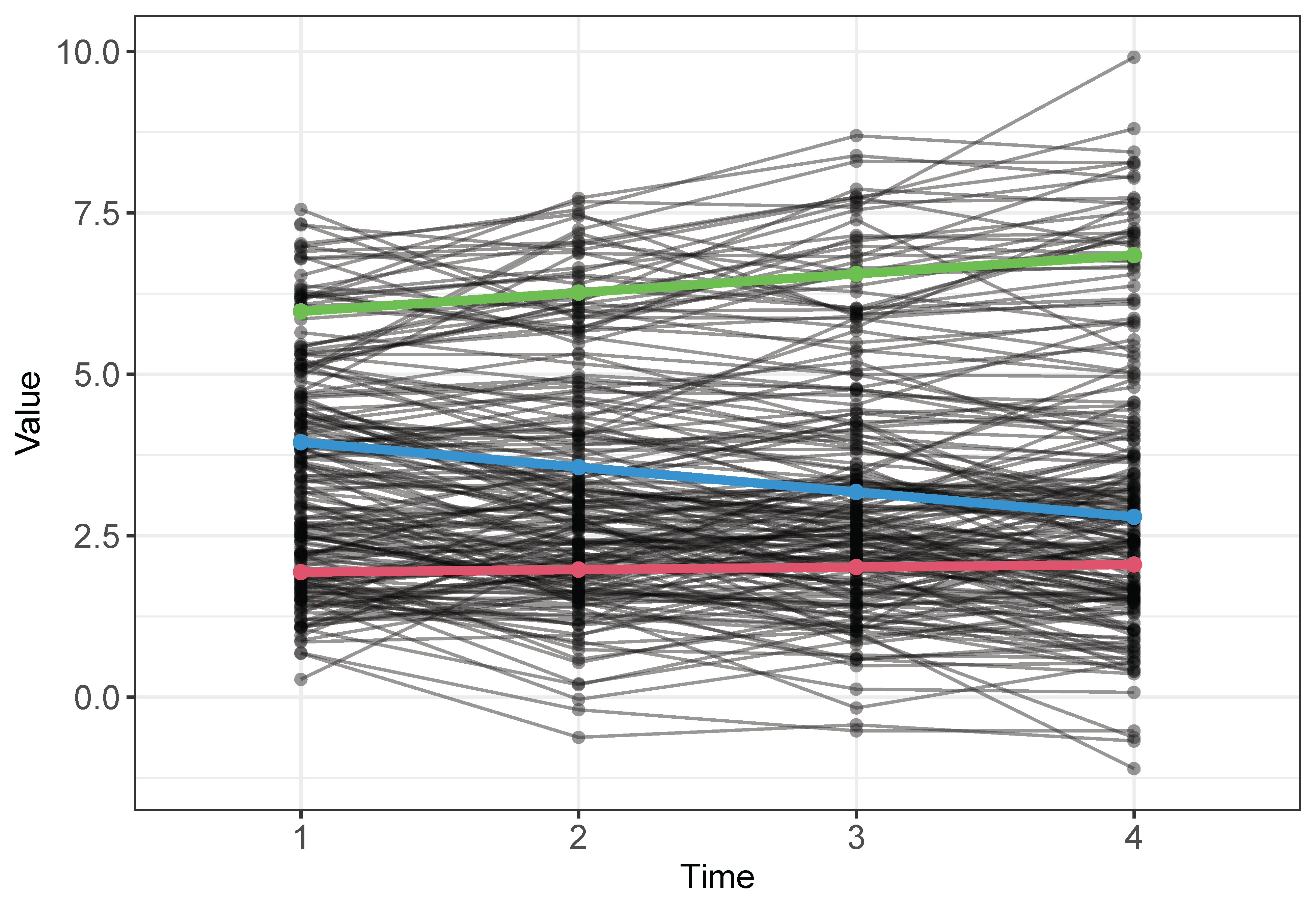
We simulate a dataset of 200 subjects from a LGMM model with 3 classes and 4 time points. The parameters shown in Table 3 serve as the population values for the data generating model. Each subject’s class membership is generated from unequal class sizes ($\boldsymbol {w}$) of 0.5, 0.3, and 0.2. Growth factor means are set to $\left (\beta _{I1}, \beta _{S1}\right )^T=(2,0)^T$ in Class 1, to $\left (\beta _{I2}, \beta _{S2}\right )^T=(4,-0.3)^T$ in Class 2, and to $\left (\beta _{I3}, \beta _{S3}\right )^T=(6,0.3)^T$ in Class 3. In addition, $\boldsymbol {\Psi }=\left (\begin {array}{cc}0.3 & 0 \\ 0 & 0.1\end {array}\right )$ and $\sigma ^2=0.5$ for the three classes.
| Class | w | $\beta _I$ | $\beta _S$ | $\Psi $ | $\sigma ^2$ |
| 1 | 0.5 | 2 | 0 | 0.3, 0, 0, 0.1 | 0.5 |
| 2 | 0.3 | 4 | -0.3 | 0.3, 0, 0, 0.1 | 0.5 |
| 3 | 0.2 | 6 | 0.3 | 0.3, 0, 0, 0.1 | 0.5 |
# Build model: latent growth mixture model
gmm <- "
model {
      #===========================
      # likelihood specification
      #===========================

      for (i in 1:N)  {
        Z[i] ~ dcat(w[1:K])
        for(t in 1:Time) {
          # model the growth curve
          y[i,t] ~ dnorm(muy[i,t], pre_sig2)
          muy[i,t] <- LS[i,1]+(t-1)*LS[i,2]
        }
        LS[i,1:2] ~ dmnorm(muLS[Z[i],1:2], Inv_cov[1:2,1:2])
      }

      #===========================
      # prior specification
      #===========================

      # --------- w ---------
        w[1:K] ~ ddirich(alpha[1:K])
        for(k in 1:K) {alpha[k] <- 1}

      # --------- muLS ---------
      for(k in 1:K) {
        # normal prior for mean of latent intercept
        muLS[k,1] ~ dnorm(0,0.001)
        # normal prior for mean of latent slope
        muLS[k,2] ~ dnorm(0,0.001)
      }

      # --------- Inv_cov ---------
      # Wishart prior for precision matrix
      Inv_cov[1:2,1:2] ~ dwish(R[1:2,1:2],2)
      Cov_b[1:2,1:2] <- inverse(Inv_cov[1:2,1:2])
      R[1,1] <- 1
      R[2,2] <- 1
      R[2,1] <- R[1,2]
      R[1,2] <- 0


      # --------- pre_sig2 ---------
      pre_sig2 ~ dgamma(0.1,0.1)   # gamma prior for precision
      sig2 <- 1/pre_sig2
}"
# Automatically generated initial values
inits <- list(".RNG.name"="base::Wichmann-Hill", ".RNG.seed"=111)
# Bundle data for JAGS
Dat <- list("y"=dat.gmm$y, "Time"=4, "N"=200, "K"=3)
# Run the analysis
set.seed(1234)
out_gmm <- run.jags(model=gmm, monitor=c(’w’,’muLS’,’Cov_b’,’sig2’),
          data=Dat, inits=inits, method="rjags", n.chains=1,
          adapt=1000, burnin=1000, sample=10000, thin=1)
Similarly, no signs of label switching are found in Figure 9.
na <- nb <- 1000
out.burn <- window(out_gmm$mcmc, start=na+nb+1)
con.diag <- geweke.diag(out.burn)
flag.noncov <- which(abs(con.diag[[1]]$z)>2)
sum.stats <- summary(out.burn)         # summary statistics
post.means <- sum.stats$statistics[,1] # posterior means
sum.stats[[1]]                         # display part 1 of the
                                       # summary statistics
##                   Mean         SD     Naive SE Time-series SE
## w[1]        0.47670814 0.04073104 0.0004073104   0.0012239491
## w[2]        0.21085352 0.03102677 0.0003102677   0.0004599641
## w[3]        0.31243835 0.03959052 0.0003959052   0.0011664481
## muLS[1,1]   1.93669961 0.08287253 0.0008287253   0.0028227498
## muLS[2,1]   5.97551073 0.12216168 0.0012216168   0.0028493240
## muLS[3,1]   3.94876895 0.12075438 0.0012075438   0.0043165390
## muLS[1,2]   0.03924477 0.04421641 0.0004421641   0.0012517566
## muLS[2,2]   0.29034785 0.06514009 0.0006514009   0.0011798124
## muLS[3,2]  -0.38549236 0.05797084 0.0005797084   0.0015226840
## Cov_b[1,1]  0.26303998 0.05820339 0.0005820339   0.0020464038
## Cov_b[2,1]  0.03346480 0.02181222 0.0002181222   0.0007339775
## Cov_b[1,2]  0.03346480 0.02181222 0.0002181222   0.0007339775
## Cov_b[2,2]  0.10267863 0.01584738 0.0001584738   0.0003574567
## sig2        0.26908279 0.01841780 0.0001841780   0.0003431461
The profiles of the classes are displayed in Figure 10.
Weller and Faubert (2020) provides guidelines on the information that should be included in an LCA report:
Another comprehensive summary table can be found in Hancock et al. (2019, p. 165), which lists key elements that should be addressed in any manuscript’s methodological approach to LCA. In addition, Depaoli (2021) provides a template for how to write up Bayesian LCA results for an empirical study (see Section 9.7, p. 340).
LCA is a popular technique that allows researchers to cluster individuals into latent classes based on response patterns to manifest variables. In this tutorial, LCA is described in a pedagogical manner to address the main challenge confronting applied researchers$-$how to transition from statistical modeling to computer programming. Although we demonstrated both the conventional LCA and its Bayesian counterpart, we put emphasis on the Bayesian side. The Bayesian framework can be advantageous for estimating LCA, particularly when sample sizes are relatively small. The use of priors can improve the ability to obtain viable and interpretable results. Nonetheless, the Bayesian approach is not exempt from pitfalls. For instance, the label switching phenomenon makes the generated MCMC samples non-identifiable and thus complicates the posterior inference. Additionally, we highlighted other issues that one should be aware of when performing LCA, including boundary estimates and quantitatively different classes.
The basic LCA for binary items along with the real data example should provide the foundation for the readers to move on smoothly to the two more advanced extensions: mixed-mode LCA and latent growth curve mixture model. In the JAGS implementation, we decomposed these modeling approaches into eight steps. Such a step-by-step procedure should allow the readers to apply similar models in practice without much difficulty. We hope that this tutorial serves as an approachable entry to a particular context of the extensive Bayesian statistics literature.
Supplementary materials can be downloaded here: https://doi.org/10.35566/jbds/v2n2/qiu.
Asparouhov, T., & Muthen, B. (2014). Auxiliary variables in mixture modeling: Three-step approaches using mplus. Structural Equation Modeling, 21(3), 329—341. doi: https://doi.org/10.1080/10705511.2014.915181
Cloitre, M., Garvert, D. W., Weiss, B., Carlson, E. B., & Bryant, R. A. (2014). Distinguishing PTSD, complex PTSD, and Borderline Personality Disorder: A latent class analysis. European Journal of Psychotraumatology, 5(1), 25097–25010. doi: https://doi.org/10.3402/ejpt.v5.25097
Collins, L. M., & Lanza, S. T. (2010). Latent class and latent transition analysis: with applications in the social behavioral, and health sciences. New Jersey: Wiley.
Depaoli, S. (2021). Bayesian structural equation modeling. New York: Guilford.
Hancock, G. R., Harring, J., & Macready, G. B. (2019). Advances in latent class analysis: A festschrift in honor of C. Mitchell Dayton. North Carolina: Information Age Publishing.
Hancock, G. R., Stapleton, L. M., & Mueller, R. O. (2019). The reviewer’s guide to quantitative methods in the social sciences (2nd ed.). New York: Routledge.
Harrington, J. M., Dahly, D. L., Fitzgerald, A. P., Gilthorpe, M. S., & Perry, I. J. (2014). Capturing changes in dietary patterns among older adults: A latent class analysis of an ageing irish cohort. Public Health Nutrition, 17(12), 2674–2686. doi: https://doi.org/10.1017/S1368980014000111
Haughton, D., Legrand, P., & Woolford, S. (2009). Review of three latent class cluster analysis packages: Latent Gold, poLCA, and MCLUST. The American Statistician, 63(1), 81—91. doi: https://doi.org/10.1198/tast.2009.0016
Linzer, D. A., & Lewis, J. (2011). poLCA: An R package for polytomous variable latent class analysis. Journal of Statistical Software, 42(10). doi: https://doi.org/10.18637/jss.v042.i10
McLachlan, G. J., & Peel, D. (2000). Finite mixture models. New Jersey: Wiley.
Merz, E. L., & Roesch, S. C. (2011). Latent profile analysis of the five factor model of personality: Modeling trait interactions. Personality and Individual Differences, 51(8), 915–919. doi: https://doi.org/10.1016/j.paid.2011.07.022
Muthen, L. K., & Muthen, B. O. (1998-2017). Mplus user’s guide (8th ed.). [Muthen and Muthen.].
O’Hagan, A., Murphy, T. B., Scrucca, L., & Gormley, I. C. (2019). Investigation of parameter uncertainty in clustering using a gaussian mixture model via jackknife, bootstrap and weighted likelihood bootstrap. Computational Statistics, 34(4), 1779–1813. doi: https://doi.org/10.1007/s00180-019-00897-9
Papastamoulis, P. (2016). label.switching: An R package for dealing with the label switching problem in MCMC outputs. Journal of Statistical Software, 69(1), 1–24.
Rosenberg, J., Beymer, P., Anderson, D., van Lissa, C. j., & Schmidt, J. (2018). tidyLPA: An R package to easily carry out latent profile analysis (LPA) using open-source or commercial software. Journal of Open Source Software, 3(30), 978. doi: https://doi.org/10.21105/joss.00978
SAS. (2016). SAS/SHARE 9.4: User’s guide. SAS Institute Inc.
Scrucca, L., Fop, M., Murphy, T. B., & Raftery, A. E. (2016). mclust 5: Clustering, classification and density estimation using Gaussian finite mixture models. The R Journal, 8(1), 289—317. doi: https://doi.org/10.32614/RJ-2016-021
STATA. (1985-2019). Stata user’s guide: Release 16. Stata Press.
Vermunt, J. K., & Magidson, J. (2016). Upgrade manual for Latent GOLD 5.1. Statistical Innovations Inc.
Weller, B. E., Bowen, N. K., & Faubert, S. J. (2020). Latent class analysis: a guide to best practice. Journal of Black Psychology, 46(4), 287—311. doi: https://doi.org/10.1177/0095798420930932
Xiao, Y., Romanelli, M., & Lindsey, M. A. (2019). A latent class analysis of health lifestyles and suicidal behaviors among US adolescents. Journal of Affective Disorders, 255, 116–126. doi: https://doi.org/10.1016/j.jad.2019.05.031
Yao, W. (2015). Label switching and its solutions for frequentist mixture models. Annual Review of Statistics and Its Application, 85(5), 1000—1012. doi: https://doi.org/10.1080/00949655.2013.859259
1 The terms mixing proportions, weights, and class sizes are used interchangeably in this tutorial.