Keywords: Missing data · Bayesian analysis· Structural equation model
The problem of missing data is prevalent in research, and the social sciences are particularly influenced by this problem because surveys are commonly used to collect information. As pointed out by Berchtold (2019), item-level missing data were found in 69.5% of papers published in selected social science journals, suggesting that the issue of missing data is quite omnipresent. Missing data may lead to various problems including biases in estimations and lowered identifiability of models (e.g., Zhang & Wang, 2012). To address missing data issues, procedures including listwise deletion, full-information maximum likelihood estimation, and multiple imputation have been proposed (e.g., Zhang & Wang, 2013). One emerging context where models can be fitted with the presence of missing data is the Bayesian framework (Ma & Chen, 2018). With Bayesian inference, missing data can be handled quite naturally. The purpose of this paper is to demonstrate the procedure of fitting a structural equation model with missing data under the Bayesian framework using the software JAGS (Plummer et al., 2003).
Three missing data mechanisms, Missing Completely at Random (MCAR), Missing at Random (MAR), and Missing Not at Random (MNAR), have been discussed in the literature (Rubin, 1976). To distinguish these mechanisms, we can use a vector \(Y\) to denote the outcome variable, a matrix \(X\) to denote the covariates, and a vector \(R\) to denote the missing data indicator for the outcome \(Y\), with \(R=1\) if a \(Y\) is missing, otherwise 0. We can also assume a model with parameter \(\gamma \) that governs the generation process of \(R\). Further, we can assume that the purpose of data analysis is to obtain the parameter \(\theta \) that explains \(Y\) using \(X\). To illustrate the different missing data mechanisms, we use missingness in the outcome \(Y\) as an example.
Under the Bayesian framework, when the missing outcome data mechanism is ignorable (MCAR or MAR), meaning that the missingness can be viewed as random after accounting for observed data, the parameter \(\theta \) of interest in the statistical analysis model can be estimated based on the observed part of data \(Y_{obs}\). For simplicity, we assume covariates \(X\) are fully observed for now. Thus, for ignorable missing outcome data, we can derive \(P(\theta |Y_{obs}, X) \propto P(Y_{obs}|\theta , X)\pi (\theta )\) as the posterior of \(\theta \) based on the observed part of data \(P(Y_{obs}|\theta , X)\) and the prior \(\pi (\theta )\). Any suitable model for the outcome variable can be used under the above scheme to obtain posterior samples of the parameter when missing data are present (Ma & Chen, 2018).
When the missing outcome data are non-ignorable (MNAR), meaning that the missingness mechanism cannot be fully explained by observed data, models such as the selection model and the pattern-mixture model can be used. Again, we assume that the covariates \(X\) are fully observed for now. When missing data are non-ignorable, the target parameter of estimation is not only \(\theta \), but both \(\theta \) and \(\gamma \).
Selection Model. The selection model partitions the joint conditional probability of the outcome variable \(Y\) and missing data indicator \(R\) into two parts: \(P(Y, R|\theta , \gamma , X)=P(Y|\theta , X)\cdot P(R|\gamma , Y, X)\) (Heckman, 1979). The part \(P(Y|\theta , X)\) denotes the probability of the outcome \(Y\) based on covariates \(X\) and parameters \(\theta \) not accounting for missingness. The part \(P(R|\gamma , Y, X)\) denotes the missingness mechanism based on both the covariates and the outcome data. While the selection model assumes the same analysis model for observed and missing data, it also assumes that the missingness indicator can be viewed as a function of the data. To incorporate the selection model into the Bayesian estimation process, we can write the posterior as \(P(\theta , \gamma |Y, X, R) \propto P(Y|\theta , X)P(R|\gamma , X, Y)\pi (\theta , \gamma )\) so that in addition to the the model parameter \(\theta \), the missing data parameter \(\gamma \) is also estimated.
Pattern-Mixture Model. The pattern-mixture model factors the joint conditional probability of the outcome \(Y\) and the missingness indicator \(R\) in a different way: \(P(Y, R|\theta , \gamma , X)=P(Y|\theta , X, R)\cdot P(R|\gamma , X)\) (Little, 1994). In this model , the part \(P(Y|\theta , X, R)\) indicates that the outcome \(Y\) depends on missingness (i.e., the outcome model could be different for observed and missing data resembling a mixture model), and the part \(P(R|\gamma , X)\) denotes the missingness mechanisms that only depend on the covariates and not on the outcome. To incorporate the pattern-mixture model into the Bayesian estimation process, we can express the posterior as \(P(\theta , \gamma |Y, X, R) \propto P(Y|\theta , X, R)P(R|\gamma , X)\pi (\theta , \gamma )\).
In Section 1.2, Bayesian schemes for handing missing data in the outcome variable are discussed assuming that the covariates are complete. However, covariates often contain missing data as well in real life. Thus, the estimation procedures need further adaptations. When the missing data mechanism for the covariates are ignorable (MCAR or MAR), distributions of the covariates can be specified in addition to the models in Section 1.2 such that each covariate can have its own conditional distribution (Ibrahim, Chen, & Lipsitz, 2002). When the missing covariates are non-ignorable (MNAR), models similar to the non-ignorable missing outcome model can also be applied to the covariates such as the selection model for both outcome and covariates implemented by Lee and Tang (2006).
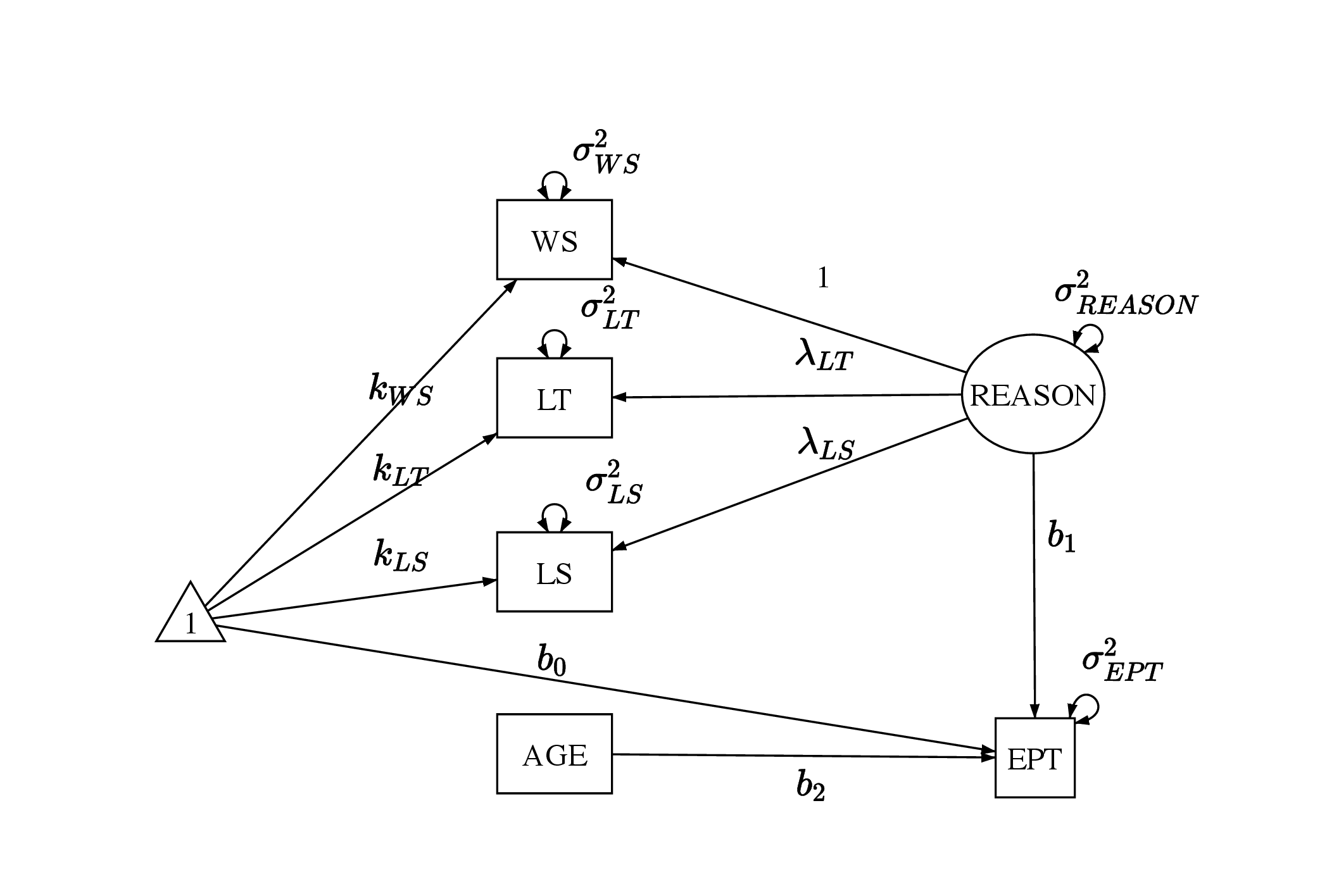
A subset of data from the The Advanced Cognitive Training for Independent and Vital Elderly (ACTIVE) study will be used to illustrate how to handle missing data under the Bayesian framework (Tennstedt et al., 2010). The dataset can be found online via https://www.icpsr.umich.edu/web/NACDA/studies/4248. A total of \(n = 500\) records for 5 variables, including 3 items measuring reasoning ability (i.e., WS, LS, and LT), AGE, and EPT will be used. Here, WS is the word series test result, LS is the letter series test result, LT is the letter sets test result, AGE is the age of participants, and EPT is the Everyday Problems Test result. The respective scores are the integer number of correct answers in each test.
The subset of data selected contains no missing values. For the purpose of this tutorial, missing values are generated according to the MAR and MNAR mechanisms. For the ignorable missingness model, 14.8% of missing data in EPT are simulated such that \(logit(P(R_i=1))= -0.6 + 0.01*Age_i\) where the \(R_i\) is the missingness indicator for the \(i\)-th record on EPT. For the selection model on handling non-ignorable missingness, 16.2% of missing data in EPT are simulated such that \(logit(P(R_i=1)) = 0.01*EPT_i\). Lastly, for the pattern mixture model on handing non-ignorable missingness, 17.6% of missing data in EPT are simulated by viewing EPT values between 24 and 26 as missing. Because EPT consists of integer values only, this means that only the EPT values of 24, 25 and 26 are missing. Thus, when viewing EPT as a linear function of other variables, which is what we will use in the analysis, the slopes for predictors will be small for missing EPT since there is very low variance in missing EPT compared to other variables; whereas for observed EPT, we can expect larger slopes. Additionally, because EPT values are mostly below 24, we can also expect the intercept for missing EPT to be larger than that of observed EPT.
The analysis model will be a structural equation model using the three reasoning ability items (i.e., WS, LS, and LT) and AGE to predict EPT as shown in Figure 1. The measurement model can be written as in Equation 1: \begin {equation} \label {eq:am1} \mathbf {X_m} = \boldsymbol {\mu } + \boldsymbol \eta \mathbf \Lambda + \boldsymbol \epsilon . \end {equation} We denote the three manifest variables that are the reasoning ability items involved in the measurement model using the matrix \(\mathbf {X_m}\) with dimension \(n \times 3\) as formatted in Equation 2. In addition, the latent variable \(REASON\) is represented by the second column in \(\boldsymbol \eta _{n \times 1}\), the factor loadings are represented by \(\mathbf \Lambda _{1 \times 3}\), the intercepts are represented by \(\boldsymbol \mu _{1 \times 3}\), and the error terms are represented by \(\boldsymbol \epsilon _{n \times 3}\). In the measurement model, it is assumed that \(\epsilon _{i1} \sim \mathcal {N}(0, \sigma _{WS}^2)\), \(\epsilon _{i2} \sim \mathcal {N}(0, \sigma _{LT}^2)\), and \(\epsilon _{i3} \sim \mathcal {N}(0, \sigma _{LS}^2)\) for \(i \in (1,...,n)\). Further, we assume the latent variable \(REASON_i \sim \mathcal {N} (0,\sigma _{REASON}^2)\).
\begin {equation} \label {eq:xm} \begin {aligned} \mathbf {X_m} &= \begin {bmatrix} WS_1 & LT_1 & LS_1\\ ... & ... & ...\\ WS_n & LT_n & LS_n\\ \end {bmatrix} \\ \boldsymbol \mu &= \begin {bmatrix} k_1 & k_2 & k_3 \end {bmatrix}\\ \boldsymbol \eta &= \begin {bmatrix} REASON_1 \\ ...\\ REASON_n \end {bmatrix}\\ \mathbf \Lambda &= \begin {bmatrix} 1 & \lambda _{LT} & \lambda _{LS} \end {bmatrix} \\ \boldsymbol \epsilon &= \begin {bmatrix} \epsilon _{11} & \epsilon _{12} & \epsilon _{13}\\ ... & ... & ... \\ \epsilon _{n1} & \epsilon _{n2} & \epsilon _{n3} \\ \end {bmatrix} \end {aligned}. \end {equation}
The structural model follows Equation 3. Since the outcome is one-dimensional, we write the structural model with respect to the outcome EPT directly. In the structural model, the latent variable REASON and the observed variable AGE are used to predict EPT with an intercept. Similar to the assumptions of the measurement model, it is assumed that \(\epsilon ^{EPT}_i \sim \mathcal {N} (0, \sigma _{EPT}^2)\).
\begin {equation} \label {eq:am3} EPT_i = b_0 + b_1 REASON_i + b_2 AGE_i + \epsilon ^{EPT}_i. \end {equation}
Together, the measurement and structural models can also be written with respect to each item as in Equation 4:
\begin {equation} \label {eq:am2} \begin {aligned} WS_i &= k_{WS} + REASON_i + \epsilon _{i1} \\ LT_i &= k_{LT} + \lambda _{LT} REASON_i + \epsilon _{i2} \\ LS_i &= k_{LS} + \lambda _{LS} REASON_i + \epsilon _{i3} \\ EPT_i &= b_0 + b_1 REASON_i + b_2 AGE_i + \epsilon ^{EPT}_i \end {aligned}. \end {equation}
Combining the measurement model and the structural model, the probability distribution function form of the analysis model used can be written as in Equation 5:
\begin {equation} \label {eq:am4} \begin {aligned} REASON_i &\sim \mathcal {N}(0, \sigma _{REASON}^2)\\ WS_i &\sim \mathcal {N}( k_{WS} + REASON_i,\sigma _{WS}^2)\\ LT_i &\sim \mathcal {N}(k_{LT} + \lambda _{LT} REASON_i,\sigma _{LT}^2)\\ LS_i &\sim \mathcal {N}(k_{LS} + \lambda _{LS} REASON_i,\sigma _{LS}^2)\\ EPT_{i} &\sim \mathcal {N}(b_0 + b_1 REASON_i + b_2 AGE_i, \sigma _{EPT}^2) \end {aligned}. \end {equation}
JAGS will be used to conduct Bayesian inference in this paper. JAGS can be installed via https://mcmc-jags.sourceforge.io/ (Plummer et al., 2003). In this paper, JAGS will be used in the R environment (R Core Team, 2021) through the software RStudio (RStudio Team, 2022) and the package runjags (Denwood, 2016). Other packages such as rjags (Plummer, Stukalov, & Denwood, 2022) that provide similar functionalities to runjags are available as well. JAGS can also be executed from the command line without using another interface.
In R, the package runjags can be installed using install.packages("runjags") and loaded using library(runjags).
In Bayesian inference with JAGS, the two crucial components to a model are the likelihood and the priors.
If the missingness in the outcome of EPT is ignorable in the data, then missing data can be addressed by sampling from the analysis model using observed data. Thus, the model in Equation 4 can be used as the ignorable missingness model. Further, the likelihood can be specified using the probability densities in Equation 5. In this example, we do not have missing data in the covariates. However, when missing data are present in the covariates, additional distributions will need to be specified for them.
We also need to specify the priors for the ignorable missingness model. Since we are using the assumption that the observed and latent variables all follow normal distributions, which is common in the practice of structural equation modeling, we can choose the priors in Equation 6 for the model parameters. In particular, the regression coefficients, factor loadings, and intercepts will have normal priors, and the variance components will have inverse gamma priors. Because there is only one latent factor in the model used, the inverse gamma distribution could satisfy as the prior for the factor variance. However, when more than one factors are involved in a structural equation model, and when the factors are allowed to correlate, the inverse wishart distribution can be used as the prior for the factor covariance matrix.
\begin {equation} \label {eq:ignorableprior} \begin {aligned} b_0, b_1, b_2 &\sim \mathcal {N} (\mu _b, \sigma ^2_b)\\ \sigma ^2_{EPT} &\sim \mathcal {IG} (h_{EPT}, \theta _{EPT})\\ \lambda _{LT}, \lambda _{LS} &\sim \mathcal {N}(\mu _{\lambda }, \sigma ^2_{\lambda })\\ \sigma ^2_{WS},\sigma ^2_{LT}, \sigma ^2_{LS} &\sim \mathcal {IG} (h_m, \theta _m)\\ k_{WS}, k_{LT}, k_{LS} &\sim \mathcal {N} (\mu _k, \sigma ^2_k)\\ \sigma ^2_{REASON} &\sim \mathcal {IG} (h_{REASON}, \theta _{REASON}) \end {aligned}. \end {equation}
In this tutorial, we will choose rather uninformative priors. But more informative priors can also be adopted. For example, the power priors can be used which constructs priors based on likelihood in historical data (Ibrahim & Chen, 2000). Hierarchical priors is another option which can be used when a range of values for the priors are available, so different levels of priors can be specified (Berger & Strawderman, 1996). These methods can be utilized for more theory-informed specification of priors.
Implementing a model in JAGS involves the following steps.
Using runjags, the model specification can be stored as a string. For example, the
code below specifies a model named ignorable.
ignorable <- "
#likelihood
...
#prior
...
"
The likelihood as specified in Section 3.1.0 can be implemented inside the model
string as the following. In JAGS, distributions can be specified using the symbol ~ .
As an illustration, in the code EPT[i] ~ dnorm(mu.EPT[i], pre.EPT), dnorm
indicates that EPT is expected to follow a normal distribution with the mean
of mu.EPT and the precision (i.e., inverse of variance) of pre.EPT. Further,
mu.EPT[i] <- b0 + b1*REASON[i] + b2*AGE[i] shows that EPT is predicted by the
latent variable REASON and the observed variable AGE. The two lines of code
together correspond to Equation 3. Note that while ~ is used to specify a
distribution, <- is used to assign values. Similar to how the distribution of EPT is
specified, the measurement model for the 3 reasoning ability items can be
specified.
# likelihood
for (i in 1:N){
  EPT[i] ~ dnorm(mu.EPT[i], pre.EPT)
  mu.EPT[i] <- b0 + b1*REASON[i] + b2*AGE[i]
  WS[i] ~ dnorm(mu1[i], pre.WS)
  LT[i] ~ dnorm(mu2[i], pre.LT)
  LS[i] ~ dnorm(mu3[i], pre.LS)
  mu1[i] <- REASON[i] + k.WS
  mu2[i] <- l.LT*REASON[i] + k.LT
  mu3[i] <- l.LS*REASON[i] + k.LS
  REASON[i] ~ dnorm(0, pre.REASON)
}
As mentioned in Section 3.1.0, historical data and previous research conclusions are not used to construct the priors here; instead, the priors used are rather uninformative. For example, the prior for means the error terms in the factor model of REASON has precision of 0.001 or variance of 1000.
# priors
# regression model
b0 ~ dnorm(0, pre.b)
b1 ~ dnorm(0, pre.b)
b2 ~ dnorm(0, pre.b)
pre.b ~ dgamma(.001,.001)
pre.EPT ~ dgamma(0.001, 0.001)

# factor model
l.LT ~ dnorm(0, 0.001)
l.LS ~ dnorm(0, 0.001)
pre.WS ~ dgamma(0.001, 0.001)
pre.LT ~ dgamma(0.001, 0.001)
pre.LS ~ dgamma(0.001, 0.001)
k.WS ~ dnorm(0, 0.001)
k.LT ~ dnorm(0, 0.001)
k.LS ~ dnorm(0, 0.001)
pre.REASON ~ dgamma(0.001, 0.001)
Additionally, to monitor the variances of various variables instead of the precision, we can use the following to convert precisions to variances.
# variances
var.EPT <- 1/pre.EPT
var.WS <- 1/pre.WS
var.LT <- 1/pre.LT
var.LS <- 1/pre.LS
var.REASON <- 1/pre.REASON
To estimate the ignorable missingness model, we define the data to be used as follows.
data <- list(N = 500,
             EPT = data_500_mar$EPT,
             AGE = data_500_mar$AGE,
             WS = data_500_mar$WS,
             LT = data_500_mar$LT,
             LS = data_500_mar$LS)
We also define initial values for the two MCMC chains that will be used. Slightly different starting values for the two chains are specified to ensure that the two chains will not converge to the same local optimum, if happening, for better convergence diagnostic.
inits <- list(list(b0=0, b1=0, b2=0, l.LT=0, l.LS=0,
                  k.WS=0, k.LS=0, k.LT=0,
                  pre.WS=0.1, pre.LS=0.1, pre.LT=0.1,
                  pre.EPT=0.1, pre.REASON=0.1),
              list(b0=1, b1=1, b2=1, l.LT=1, l.LS=1,
                  k.WS=1, k.LS=1, k.LT=1,
                  pre.WS=0.2, pre.LS=0.2, pre.LT=0.2,
                  pre.EPT=0.2, pre.REASON=0.2))
Finally, the posteriors can be sampled using the run.jags command. The
model=ignorable argument specifies that the model named m1 will be used. The
monitor argument specifies which parameters or variables we want to sample. The
data=data, n.chains=2, inits=inits arguments specify the data, number of chains,
and initial values to be used, respectively. The arguments adapt=1000, burnin = 3000,
and sample=100000 specify the number of adaptation, burn-in, and sampling
iterations, respectively. Only the sampling iterations will be recorded. The argument
keep.jags.files=FALSE instructs JAGS to not save any files produced in the
sampling process. If the argument is set to keep.jags.files=FALSE, then additional
files will be saved in a folder named runjagsfiles. The argument thin=1 sets the
intervals of recorded samples to be 1, meaning that every iteration will be saved. The
argument method="simple" indicates that the simple method would be used
to compile the model. The argument tempdir=TRUE asks JAGS to create
a temporary directory to store files instead of saving files in the working
directory.
out1 <- run.jags(model=ignorable,
                 monitor=c("b0", "b1", "b2",
                "l.LT", "l.LS",
                "k.WS", "k.LT", "k.LS",
                "var.WS", "var.LT",
                "var.LS", "var.EPT", "var.REASON"),
                 data=data, n.chains=2,
                 inits=inits, method="simple",
                 adapt=1000, burnin = 3000,
                 sample=1000000,
                 thin=1,
                 keep.jags.files=FALSE,
                 tempdir=TRUE)
The summary(out1) command in runjags gives the summary statistics of the JAGS
output which can be used for convergence diagnostics. We will mainly rely on the
Gelman-Rubin test for diagnosing convergence (Gelman & Rubin, 1992).
The Gelman-Rubin test statistics, or the potential scale reduction factor, is
readily provided by the summary function and is suitable when multiple chains
are used. As shown in Table 1, the potential scale reduction factors (psrf)
for all parameters are below 1.1 and very close to 1, suggesting that the
chains have converged. Monte Carlo SEs of most parameters (MCerr) are
quite low as well (\(<0.05\)). The effective sample sizes (SSeff) are also acceptable
(\(> 400\)).
| Lower95 | Median | Upper95 | Mean | MCerr | SSeff | psrf | |
| b0 | 10.546 | 16.071 | 21.450 | 16.045 | 0.041 | 4515 | 1 |
| b1 | 0.855 | 0.960 | 1.062 | 0.960 | 0.000 | 16217 | 1 |
| b2 | -0.038 | 0.034 | 0.110 | 0.034 | 0.001 | 4485 | 1 |
| l.LT | 0.402 | 0.445 | 0.489 | 0.445 | 0.000 | 20000 | 1 |
| l.LS | 1.066 | 1.142 | 1.222 | 1.142 | 0.000 | 20000 | 1 |
| k.WS | 9.266 | 9.700 | 10.129 | 9.701 | 0.002 | 20000 | 1 |
| k.LT | 5.439 | 5.684 | 5.926 | 5.683 | 0.001 | 20000 | 1 |
| k.LS | 9.744 | 10.225 | 10.726 | 10.226 | 0.002 | 20483 | 1 |
| var.WS | 3.294 | 4.247 | 5.265 | 4.260 | 0.004 | 20000 | 1 |
| var.LT | 3.025 | 3.487 | 3.995 | 3.497 | 0.002 | 20000 | 1 |
| var.LS | 3.717 | 4.981 | 6.230 | 4.994 | 0.005 | 19548 | 1 |
| var.EPT | 12.649 | 14.831 | 17.112 | 14.884 | 0.008 | 20000 | 1 |
| var.REASON | 17.037 | 19.849 | 23.122 | 19.903 | 0.011 | 20000 | 1 |
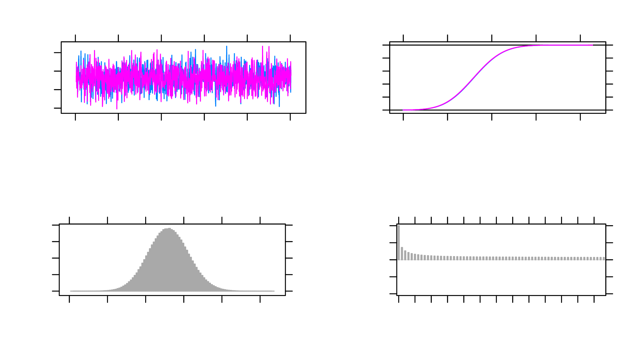
The plot(out1) command can be used to generate trace plots and histograms of
the MCMC chains which can further help diagnose the convergence of the
target parameters. For example, Figure 2 shows the MCMC plots of the
parameter \(b_1\), and the trace plot and histogram both indicate that the parameter
converged. The histogram is centered at one mode, and the trace plot looks
stable.
There are other approaches for diagnosing convergence which will not be discussed in depth here. For example, the Geweke test can be conducted using the coda package (Plummer, Best, Cowles, & Vines, 2006). This test takes two proportions of a Markov chain and applies a z-test to see if the two proportions are different. The Herdelberger and Welch test can also be used with coda which tests if the samples come from a stable distribution.
Using the Highest Posterior Density (HPD) intervals which are indicated by the Lower95 and Upper95 values in Table 1, we can see that the factor loadings and intercepts in the measurement model are likely non-zero as the HPD intervals for them excludes 0. Thus, the items WS, LT and LS do have commonalities explained by the construct of reasoning ability. In the structural model, the intercept term and the slope for REASON have their HPD intervals excluding 0, suggesting that we can conclude that the latent variable of REASON explains the variance in EPT, whereas AGE does not.
When the missingness in the outcome is MNAR or non-ignorable, the selection model can be applied. For non-ignorable missing outcome, we also make the same assumption that the missing covariates are ignorable so that we can specify conditional distributions for them. We also assume that the missingness is dependent on the outcome of EPT scores themselves in the selection model. Using a missing data indicator \(R_{i}\) where \(R_{i}=1\) denotes a missing record of EPT and \(R_{i}=0\) denotes an observed record of EPT, the selection model translates to Equation 7, which can be used in addition to the model specification in Equation 4:
\begin {equation} \label {eq:sm1} logit(P(R_{i}=1)) = a_0 + a_1 EPT_{i}. \end {equation}
The corresponding probability density distribution form of the selection model incorporates Equation 8 in addition to Equation 5:
\begin {equation} \label {eq:sm2} R_{i} \sim \mathcal {B}(sigmoid(a_0 + a_1 EPT_{i})). \end {equation}
The missing data indicator \(R_{i}\) is deemed as a function of the outcome value \(EPT_i\) and an intercept. The intercept \(a_0\) here is used to adjust the threshold for 1 and 0 in the missing data indicator of \(R_{i}\).
The priors can be constructed similarly to the ignorable missingness model. Priors for the parameters \(a_0\) and \(a_1\) are needed for the selection model as indicated by Equation 9, which can be combined with the priors in Equation 6 to be used in JAGS.
\begin {equation} \label {eq:smprior} a_0, a_1\sim \mathcal {N} (\mu _a, \sigma ^2_a) \end {equation}
In JAGS, the likelihood for the ignorable data model can be modified to incorporate the selection model by including the following.
R[i] ~ dbern(p[i])
logit(p[i]) = a0 + a1*EPT[i]
The priors also need to be modified based on the the function of missingness on EPT.
a0 ~ dnorm(0, pre.a)
a1 ~ dnorm(0, pre.a)
pre.a ~ dgamma(.001,.001)
Since the model has now changed, the initial values and data supplied should be
modified accordingly. A missing data indicator for the outcome is also needed as
shown below in the variable R = is.na(data_500_mnar$EPT)*1.
data <- list(N = 500,
             EPT = data_500_mnar$EPT,
             AGE = data_500_mnar$AGE,
             WS = data_500_mnar$WS,
             LT = data_500_mnar$LT,
             LS = data_500_mnar$LS,
             R = is.na(data_500_mnar$EPT)*1)

inits <- list(list(b0=0, b1=0, b2=0, l.LT=0, l.LS=0,
                   k.WS=0, k.LS=0, k.LT=0,
                   pre.WS=0.1, pre.LS=0.1, pre.LT=0.1,
                   pre.EPT=0.1, pre.REASON=0.1,
                   a0=0.1, a1=0.1),
              list(b0=1, b1=1, b2=1, l.LT=1, l.LS=1,
                   k.WS=1, k.LS=1, k.LT=1,
                   pre.WS=0.2, pre.LS=0.2, pre.LT=0.2,
                   pre.EPT=0.2, pre.REASON=0.2,
                   a0=0.2, a1=0.2))
The model can then be estimated using the following statement. Again, 1000 adaptation iterations, 3000 burn-in iterations, and 100000 sampling iterations are specified.
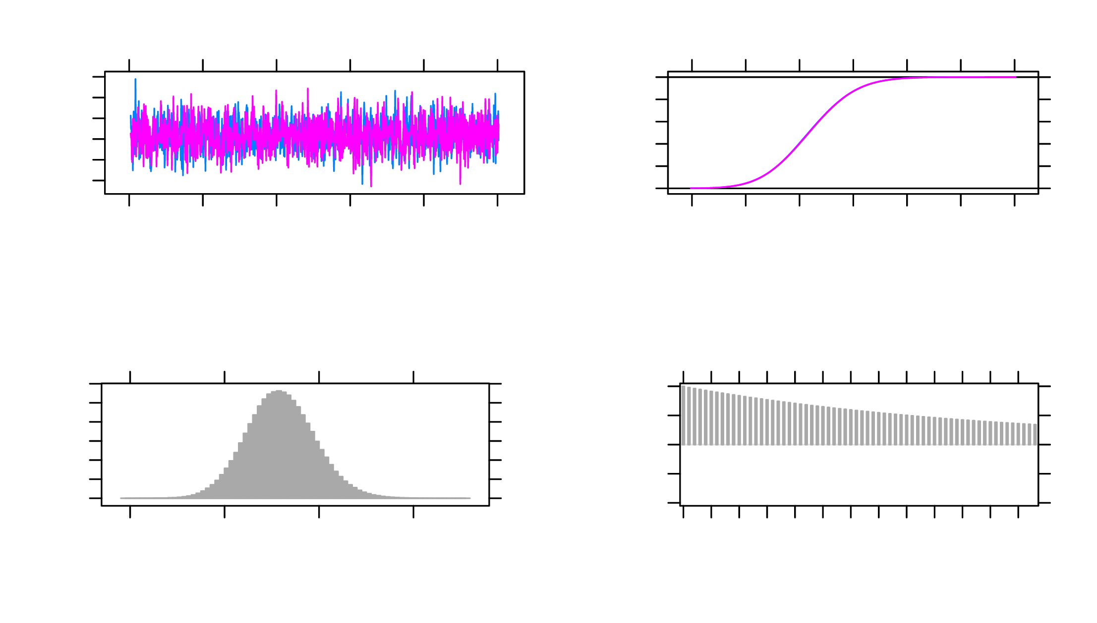
out1 <- run.jags(model=selection,
                 monitor=c("b0", "b1", "b2",
                 "a0", "a1",
                 "l.LT", "l.LS", "k.WS",
                 "k.LT", "k.LS",
                 "var.WS", "var.LT",
                 "var.LS", "var.EPT", "var.REASON"),
                 data=data, n.chains=2,
                 inits=inits, method="simple",
                 adapt=1000, burnin = 3000,
                 sample=1000000,
                 thin=1,
                 keep.jags.files=FALSE,
                 tempdir=TRUE)
As show in Table 2, the potential scale reduction factors (psrf) are all below 1.1, and the Monte Carlo SEs (MCerr) are satisfactory (\(<0.05\)). The effective sample sizes (SSeff) for all parameters are also above 400. The trace plots are satisfactory as well. As an example, MCMC plots for the parameter \(a_1\) is shown in Figure 3.
| Lower95 | Median | Upper95 | Mean | MCerr | SSeff | psrf | |
| b0 | 13.170 | 18.649 | 24.029 | 18.623 | 0.043 | 4048 | 1 |
| b1 | 0.865 | 0.968 | 1.077 | 0.968 | 0.000 | 15546 | 1 |
| b2 | -0.074 | -0.002 | 0.072 | -0.002 | 0.001 | 4064 | 1 |
| a0 | -4.276 | -2.752 | -1.374 | -2.788 | 0.006 | 13872 | 1 |
| a1 | -0.010 | 0.059 | 0.132 | 0.059 | 0.000 | 13990 | 1 |
| l.LT | 0.402 | 0.446 | 0.491 | 0.446 | 0.000 | 20000 | 1 |
| l.LS | 1.076 | 1.153 | 1.233 | 1.154 | 0.000 | 20551 | 1 |
| k.WS | 9.266 | 9.702 | 10.133 | 9.702 | 0.002 | 20000 | 1 |
| k.LT | 5.445 | 5.685 | 5.926 | 5.685 | 0.001 | 19607 | 1 |
| k.LS | 9.747 | 10.230 | 10.720 | 10.228 | 0.002 | 19719 | 1 |
| var.WS | 3.436 | 4.448 | 5.453 | 4.459 | 0.004 | 20000 | 1 |
| var.LT | 3.048 | 3.502 | 4.014 | 3.513 | 0.002 | 21125 | 1 |
| var.LS | 3.443 | 4.699 | 5.955 | 4.711 | 0.005 | 20000 | 1 |
| var.EPT | 12.945 | 15.249 | 17.670 | 15.308 | 0.009 | 19667 | 1 |
| var.REASON | 16.618 | 19.644 | 22.728 | 19.701 | 0.011 | 20000 | 1 |
Using the HPD intervals, the factor loadings and factor intercepts in the measurement model are again non-zero, indicating that the three items measuring REASON do have overlaps. In the structural part of the selection model, the intercept and the slope for the latent variable REASON both have HPD intervals excluding 0, suggesting that REASON do explain significant variance in EPT after accounting for the missingness mechanism. However, the HPD interval for the slope of AGE still contains 0, suggesting that AGE may not be a useful predictor of EPT here.
The slope for EPT in explaining the missingness mechanism has HPD intervals containing 0, suggesting that EPT’s effect on explaining missingness is small. Whereas the intercept for predicting missingness has its HPD interval excluding 0. This deviates from the data generation model because the coefficients used in missing data generation are quite small.
Although the selection model is most commonly used when missing data are
non-ignorable, it can be applied to MCAR and MAR data as well. In the ACTIVE
example, missingness predictors can be changed to, for instance, logit(p[i]) = a0 for
MCAR missingness and logit(p[i]) = a0 + a1*AGE[i] for MAR missingness, for
example.
A pattern-mixture model can also be used to handle non-ignorable missing data in
the outcome of EPT. In this case, the intercept b0 and the slope b1 for the outcome
regressed on the latent variable of REASON are deemed different for missing and
observed data, whereas in practice, theories should be used to guide the decision
on the missing data model. The pattern-mixture property is shown as the
subscripts \(R_i\) on \(b_0\) and \(b_1\) in Equation 10, which can be used in addition to the
model specification in Equation 4 as the specification for the pattern-mixture
model:
\begin {equation} \label {eq:pmm1} EPT_i = b_0^{R_i} + b_1^{R_i} REASON_i + b_2 AGE_i + \epsilon ^{EPT}_i. \end {equation}
Also, Equation 11 can be used in addition to Equation 5 as the probability density function form of the pattern-mixture model:
\begin {equation} \label {eq:pmm2} EPT_{i} \sim N(b_0^{R_i} + b_1^{R_i} REASON_i + b_2 AGE_i, \sigma _y^2). \end {equation}
Assuming \(R_i=1\) for a missing record on EPT and \(R_i=0\) for an observed record on EPT, then there are two sets of distinct \(b_0\) and \(b_1\) values for \(R_i=1\) and \(R_i=0\), respectively. It should be noted that this is merely one possible pattern-mixture model that can be fitted onto the data, and that other pattern-mixture models can be used based on specific theories.
Priors for the pattern-mixture model can be specified using Equation 12 to replace the corresponding regression coefficients priors in Equation 6. Different from the priors for the ignorable missingness model, here, priors for \(b_0\) and \(b_1\) are differentiated for missing data (\(b_0^1, b_1^1\)) and for observed data (\(b_0^0, b_1^0\)).
\begin {equation} \label {eq:pmmprior} \begin {gathered} b_0^0, b_0^1, b_1^0, b_1^1 \sim \mathcal {N} (\mu _b, \sigma ^2_b) \end {gathered} \end {equation}
Different from the ignorable missingness model, we need to specify the
mean of EPT to be different for missing and observed data such as
mu.EPT[i] <- b0[R[i]+1] + b1[R[i]+1] *REASON[i] + b2*AGE[i] in JAGS. Since JAGS
uses 1-based indexes instead of 0-based indexes, we need to use R[i]+1 instead of
R[i] in the code to transform the 0 and 1 values in the missing value indicator to 1
and 2. We also need to modify the priors of b0 and b1 as the following which is based
on the assumption that while the intercept is larger for missing EPT, the slope is
smaller for missing EPT. This assumption is based on how missing data is
generated.
  b0[1] ~ dnorm(0, pre.b) # non-missing
  b0[2] ~ dnorm(b0[1]+05, pre.b) #missing
  b1[1] ~ dnorm(0, pre.b) # non-missing
  b1[2] ~ dnorm(b1[1]-0.5, pre.b) #missing
Similar to the case in the selection model, an indicator for missing or observed data is required for estimating the pattern-mixture model, and the data statement can take the form of the following:
data <- list(N = 500,
             EPT = data_500_mnar_2$EPT,
             AGE = data_500_mnar_2$AGE,
             WS = data_500_mnar_2$WS,
             LT = data_500_mnar_2$LT,
             LS = data_500_mnar_2$LS,
             R = is.na(data_500_mnar_2$EPT)*1)
The initial values can be specified based on the pattern-mixture model. Compared
to the ignorable missingness model, initial values for b0 and b1 are changed
to incorporate two cases for missing and observed data. For example, in
the first chain, initial values for b0 and b1 are b0=c(0,1), b1=c(1,0). This
is consistent with our expectation that the intercept and slope for missing
data would be greater and lower, respectively, than those of the observed
data.
inits <- list(list(b0=c(0,1), b1=c(1,0), b2=0,
                   l.LT=0, l.LS=0, k.WS=0,
                   k.LS=0, k.LT=0,
                   pre.WS=0.1, pre.LS=0.1, pre.LT=0.1,
                   pre.EPT=0.1, pre.REASON=0.1),
              list(b0=c(1,2), b1=c(2,1), b2=1,
                   l.LT=1, l.LS=1, k.WS=1,
                   k.LS=1, k.LT=1,
                   pre.WS=0.2, pre.LS=0.2, pre.LT=0.2,
                   pre.EPT=0.2, pre.REASON=0.2))
Finally, the model can be estimated using the statement below.
out1 <- run.jags(model=pmm,
                 monitor=c("b0", "b1", "b2",
                "l.LT", "l.LS", "k.WS",
                "k.LT", "k.LS", "var.WS", "var.LT",
                "var.LS", "var.EPT", "var.REASON"),
                 data=data, n.chains=2,
                 inits=inits, method="simple",
                 adapt=1000, burnin = 3000,
                 sample=1000000,
                 thin=1,
                 keep.jags.files=FALSE,
                 tempdir=TRUE)
In Table 3 which contains the output from this model, the potential scale reduction factors (psrf) are lower than 1.1, suggesting that the chains have converged. The effective sample sizes (SSeff) are acceptable (\(>400\)), and the Monte Carlo SEs (MCerr) are mostly below 0.05.
| Lower95 | Median | Upper95 | Mean | MCerr | SSeff | psrf | |
| b0[1] | 11.522 | 16.352 | 21.157 | 16.361 | 0.034 | 5190 | 1.00 |
| b0[2] | -7.595 | 21.045 | 52.908 | 21.498 | 0.113 | 20000 | 1.00 |
| b1[1] | 0.847 | 0.950 | 1.053 | 0.951 | 0.000 | 17588 | 1.00 |
| b1[2] | -30.761 | 0.527 | 29.239 | 0.586 | 0.119 | 20000 | 1.01 |
| b2 | -0.046 | 0.020 | 0.084 | 0.020 | 0.000 | 5211 | 1.00 |
| l.LT | 0.399 | 0.443 | 0.486 | 0.443 | 0.000 | 20000 | 1.00 |
| l.LS | 1.066 | 1.141 | 1.222 | 1.142 | 0.000 | 19925 | 1.00 |
| k.WS | 9.288 | 9.705 | 10.149 | 9.705 | 0.002 | 20328 | 1.00 |
| k.LT | 5.450 | 5.686 | 5.925 | 5.686 | 0.001 | 19697 | 1.00 |
| k.LS | 9.741 | 10.232 | 10.716 | 10.231 | 0.002 | 20291 | 1.00 |
| var.WS | 3.254 | 4.204 | 5.240 | 4.218 | 0.004 | 20000 | 1.00 |
| var.LT | 3.070 | 3.524 | 4.036 | 3.533 | 0.002 | 20000 | 1.00 |
| var.LS | 3.711 | 4.955 | 6.239 | 4.968 | 0.005 | 20000 | 1.00 |
| var.EPT | 11.269 | 13.222 | 15.379 | 13.268 | 0.007 | 20000 | 1.00 |
| var.REASON | 16.956 | 19.852 | 23.114 | 19.932 | 0.011 | 20000 | 1.00 |
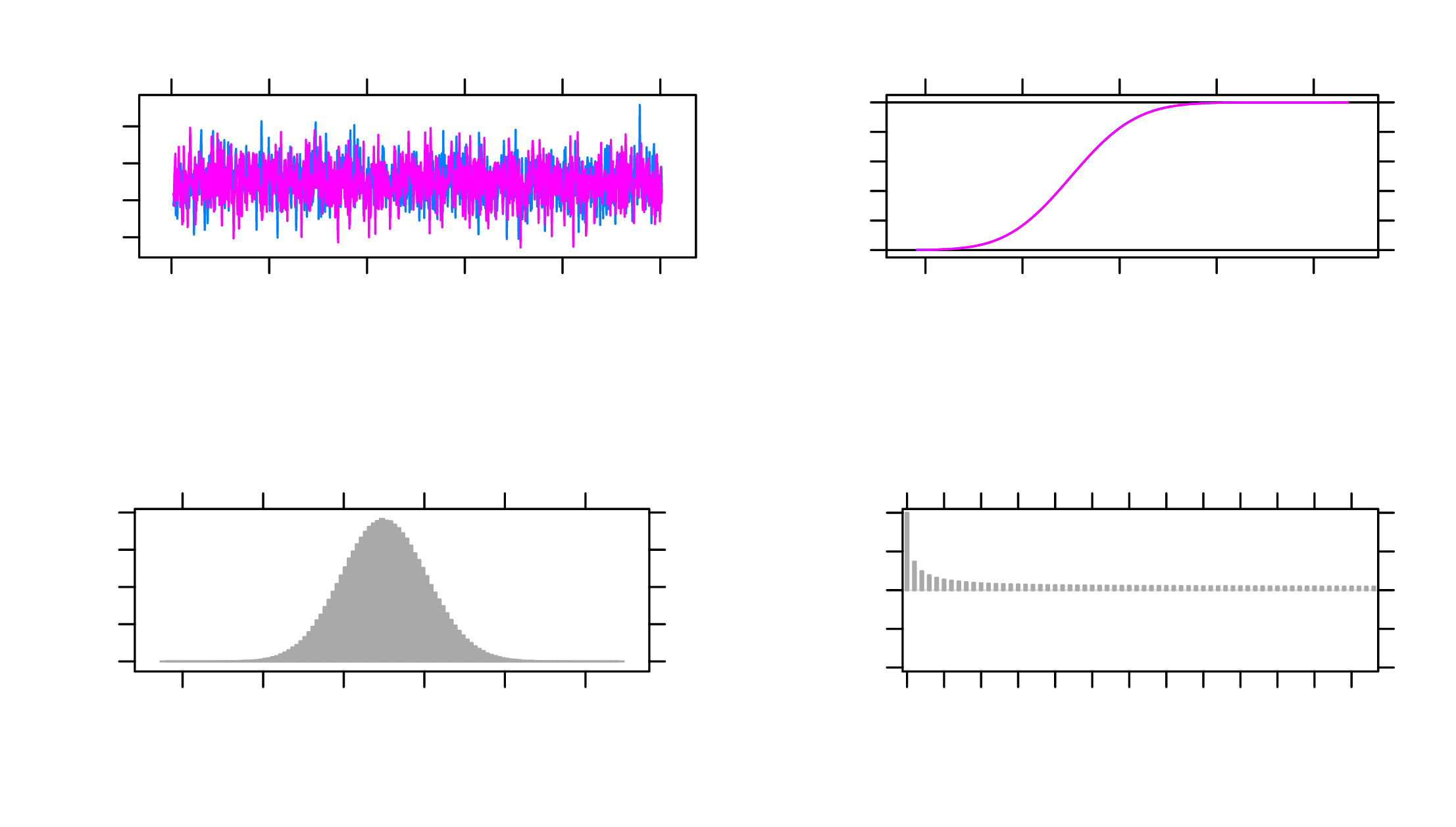
The MCMC plots in Figure 4 can also be used to diagnose convergence. Here, the
plot for b1 when data are observed is used as an example. All parameters, similar to
b1, present satisfactory trace plots suggesting that convergence is reached and the
estimates are stable.
As shown by the HPD intervals in Table 3, the factor loadings and intercepts in the measurement model again exhibit HPD intervals that exclude 0. In the structural model, AGE’s HPD interval contains 0, whereas the intercept and the slope for REASON have HPD intervals excluding 0 for observed data and including 0 for missing data. Consequently, for observed data, REASON can predict EPT whereas for missing data it is not the case.
Data with missing values can still be used for parameter estimation in different models under the Bayesian framework. In this paper, a structural equation model is used as an example on the ACTIVE study data to illustrate how models with missing data can be fitted using JAGS in R under different missing data mechanisms including MCAR, MAR, and MNAR. Specifically, two models, the selection model and the pattern-mixture model, are introduced for non-ignorable (i.e., MNAR) missing data.
While this paper mainly focuses on obtaining parameter estimates when missing data are present, other aspects of missing data are not covered here. Although not discussed in this paper, other models for handling non-ignorable missingness exist such as the shared-parameter model (Albert & Follmann, 2008). In addition, there are model selection methods for deciding which of many potential missing data models would suit the data best. For example, in sensitivity analysis which is often used to validate missing data handling processes by assessing robustness of imputations under different conditions, Bayesian model comparison criteria such as the deviation information criterion (DIC) can be used to choose the best model (Ma & Chen, 2018; Van Buuren, 2018). Further, there are ways to diagnose missing data mechanisms in a dataset such as discussed in Little (1988). These topics can be further explored.
There are also different analysis models tailored toward specific types of data that can be incorporated in Bayesian missing data handling processes, which we did not discuss in this paper. While this paper uses a structural equation model as an example, other models can be similarly constructed in JAGS to accommodate missing data. For example, longitudinal data can be analyzed using a multilevel model (Gelman & Hill, 2006). If the response data are of mixed types from mixed populations, then mixture models may be appropriate (Rasmussen, 1999). Social network data can also be used with methods such as the exponential random graph model and the latent space model (Hoff, Raftery, & Handcock, 2002; Robins, Pattison, Kalish, & Lusher, 2007). These models have Bayesian variants that can be applied to estimate parameters when missing data are present (Bürkner, 2017; Koskinen, Robins, Wang, & Pattison, 2013; Neal, 1992).
The research reported here was supported, in whole or in part, by the Institute of Education Sciences, U.S. Department of Education, through grant R305D210023 to University of Notre Dame. The opinions expressed are those of the authors and do not represent the views of the Institute or the U.S. Department of Education.
Albert, P. S., & Follmann, D. A. (2008). Shared-parameter models. In Longitudinal data analysis (pp. 447–466). Chapman and Hall/CRC. doi: https://doi.org/10.1201/9781420011579.ch19
Berchtold, A. (2019). Treatment and reporting of item-level missing data in social science research. International Journal of Social Research Methodology, 22(5), 431–439. doi: https://doi.org/10.1080/13645579.2018.1563978
Berger, J. O., & Strawderman, W. E. (1996). Choice of hierarchical priors: Admissibility in estimation of normal means. The Annals of Statistics, 931–951. doi: https://doi.org/10.1214/aos/1032526950
Bürkner, P.-C. (2017). Advanced bayesian multilevel modeling with the r package brms. arXiv preprint arXiv:1705.11123. doi: https://doi.org/10.32614/rj-2018-017
Denwood, M. J. (2016). runjags: An r package providing interface utilities, model templates, parallel computing methods and additional distributions for mcmc models in jags. Journal of statistical software, 71, 1–25. doi: https://doi.org/10.18637/jss.v071.i09
Gelman, A., & Hill, J. (2006). Data analysis using regression and multilevel/hierarchical models. Cambridge university press. doi: https://doi.org/10.1017/cbo9780511790942
Gelman, A., & Rubin, D. B. (1992). Inference from iterative simulation using multiple sequences. Statistical science, 457–472. doi: https://doi.org/10.1214/ss/1177011136
Heckman, J. J. (1979). Sample selection bias as a specification error. Econometrica: Journal of the econometric society, 153–161. doi: https://doi.org/10.2307/1912352
Hoff, P. D., Raftery, A. E., & Handcock, M. S. (2002). Latent space approaches to social network analysis. Journal of the american Statistical association, 97(460), 1090–1098. doi: https://doi.org/10.1198/016214502388618906
Ibrahim, J. G., & Chen, M.-H. (2000). Power prior distributions for regression models. Statistical Science, 46–60. doi: https://doi.org/10.1214/ss/1009212673
Ibrahim, J. G., Chen, M.-H., & Lipsitz, S. R. (2002). Bayesian methods for generalized linear models with covariates missing at random. Canadian Journal of Statistics, 30(1), 55–78. doi: https://doi.org/10.2307/3315865
Koskinen, J. H., Robins, G. L., Wang, P., & Pattison, P. E. (2013). Bayesian analysis for partially observed network data, missing ties, attributes and actors. Social networks, 35(4), 514–527. doi: https://doi.org/10.1016/j.socnet.2013.07.003
Lee, S.-Y., & Tang, N.-S. (2006). Analysis of nonlinear structural equation models with nonignorable missing covariates and ordered categorical data. Statistica Sinica, 1117–1141.
Little, R. J. (1988). A test of missing completely at random for multivariate data with missing values. Journal of the American statistical Association, 83(404), 1198–1202. doi: https://doi.org/10.1080/01621459.1988.10478722
Little, R. J. (1994). A class of pattern-mixture models for normal incomplete data. Biometrika, 81(3), 471–483. doi: https://doi.org/10.1093/biomet/81.3.471
Ma, Z., & Chen, G. (2018). Bayesian methods for dealing with missing data problems. Journal of the Korean Statistical Society, 47(3), 297–313. doi: https://doi.org/10.1016/j.jkss.2018.03.002
Neal, R. M. (1992). Bayesian mixture modeling. In Maximum entropy and bayesian methods (pp. 197–211). Springer. doi: https://doi.org/10.1007/978-94-017-2219-3_14
Plummer, M., Best, N., Cowles, K., & Vines, K. (2006). Coda: convergence diagnosis and output analysis for mcmc. R news, 6(1), 7–11.
Plummer, M., et al. (2003). Jags: A program for analysis of bayesian graphical models using gibbs sampling. In Proceedings of the 3rd international workshop on distributed statistical computing (Vol. 124, pp. 1–10).
Plummer, M., Stukalov, A., & Denwood, M. (2022). rjags: Bayesian graphical models using mcmc [Computer software manual].
R Core Team. (2021). R: A language and environment for statistical computing [Computer software manual]. Vienna, Austria. Retrieved from https://www.R-project.org/
Rasmussen, C. (1999). The infinite gaussian mixture model. Advances in neural information processing systems, 12.
Robins, G., Pattison, P., Kalish, Y., & Lusher, D. (2007). An introduction to exponential random graph (p*) models for social networks. Social networks, 29(2), 173–191. doi: https://doi.org/10.1016/j.socnet.2006.08.002
RStudio Team. (2022). Rstudio: Integrated development environment for r [Computer software manual]. Boston, MA. Retrieved from http://www.rstudio.com/
Rubin, D. B. (1976). Inference and missing data. Biometrika, 63(3), 581–592. doi: https://doi.org/10.1093/biomet/63.3.581
Tennstedt, S., Morris, J., Unverzagt, F., Rebok, G. W., Willis, S. L., Ball, K., & Marsiske, M. (2010, June 30). Advanced cognitive training for independent and vital elderly (active), united states, 1999–2001. Inter-university Consortium for Political and Social Research [distributor]. Retrieved from https://doi.org/10.3886/ICPSR04248.v3 doi: https://doi.org/10.3886/ICPSR04248.v3
Van Buuren, S. (2018). Flexible imputation of missing data. CRC press.
Zhang, Z., & Wang, L. (2012). A note on the robustness of a full bayesian method for nonignorable missing data analysis. Brazilian Journal of Probability and Statistics, 26(3), 244–264. doi: https://doi.org/10.1214/10-bjps132
Zhang, Z., & Wang, L. (2013). Methods for mediation analysis with missing data. Psychometrika, 78(1), 154–184. doi: https://doi.org/10.1007/s11336-012-9301-5
set.seed(10)
data = read.csv("active.csv")
data = data[, c("WS_COR", "LS_COR", "LT_COR",
            "AGE", "EPT")]
data = na.omit(data)
data_500 <- data[sample(nrow(data),500), ]
colnames(data_500) <- c("WS", "LS", "LT", "AGE", "EPT")

# MAR
miss <- rep(NA, nrow(data_500))
for (i in 1:nrow(data_500)){
  miss[i] <- rbinom(1, 1, data_500$AGE[i]*0.01-60*0.01)
}
data_500_mar <- data_500
data_500_mar[,"EPT"][miss==1] <- NA
summary(data_500_mar)


# MNAR selection
miss2 <- rep(NA, nrow(data_500))
for (i in 1:nrow(data_500)){
  miss2[i] <- rbinom(1, 1, data_500$EPT[i]*0.01)
}
data_500_mnar <- data_500
data_500_mnar[,"EPT"][miss2==1] <- NA
summary(data_500_mnar)

# MNAR pattern-mixture
miss3 <- rep(0, nrow(data_500))
miss3[(data_500$EPT>23) & (data_500$EPT<27)] <- 1
data_500_mnar_2 <- data_500
data_500_mnar_2[,"EPT"][miss3==1] <- NA
summary(data_500_mnar_2)
library(runjags)

ignorable <- "
model{
  # likelihood
  for (i in 1:N){
    EPT[i] ~ dnorm(mu.EPT[i], pre.EPT)
    mu.EPT[i] <- b0 + b1*REASON[i] + b2*AGE[i]
    WS[i] ~ dnorm(mu1[i], pre.WS)
    LT[i] ~ dnorm(mu2[i], pre.LT)
    LS[i] ~ dnorm(mu3[i], pre.LS)
    mu1[i] <- REASON[i] + k.WS
    mu2[i] <- l.LT*REASON[i] + k.LT
    mu3[i] <- l.LS*REASON[i] + k.LS
    REASON[i] ~ dnorm(0, pre.REASON)
  }

  # priors
  # regression model
  b0 ~ dnorm(0, pre.b)
  b1 ~ dnorm(0, pre.b)
  b2 ~ dnorm(0, pre.b)
  pre.b ~ dgamma(.001,.001)
  pre.EPT ~ dgamma(0.001, 0.001)

  # factor model
  l.LT ~ dnorm(0, 0.001)
  l.LS ~ dnorm(0, 0.001)
  pre.WS ~ dgamma(0.001, 0.001)
  pre.LT ~ dgamma(0.001, 0.001)
  pre.LS ~ dgamma(0.001, 0.001)
  k.WS ~ dnorm(0, 0.001)
  k.LT ~ dnorm(0, 0.001)
  k.LS ~ dnorm(0, 0.001)
  pre.REASON ~ dgamma(0.001, 0.001)

  # variances
  var.EPT <- 1/pre.EPT
  var.WS <- 1/pre.WS
  var.LT <- 1/pre.LT
  var.LS <- 1/pre.LS
  var.REASON <- 1/pre.REASON
}

"
data <- list(N = 500,
             EPT = data_500_mar$EPT,
             AGE = data_500_mar$AGE,
             WS = data_500_mar$WS,
             LT = data_500_mar$LT,
             LS = data_500_mar$LS)

inits <- list(list(b0=0, b1=0, b2=0, l.LT=0, l.LS=0,
                  k.WS=0, k.LS=0, k.LT=0,
                  pre.WS=0.1, pre.LS=0.1, pre.LT=0.1,
                  pre.EPT=0.1, pre.REASON=0.1),
              list(b0=1, b1=1, b2=1, l.LT=1, l.LS=1,
                  k.WS=1, k.LS=1, k.LT=1,
                  pre.WS=0.2, pre.LS=0.2, pre.LT=0.2,
                  pre.EPT=0.2, pre.REASON=0.2))

out1 <- run.jags(model=ignorable,
                 monitor=c("b0", "b1", "b2",
                "l.LT", "l.LS",
                "k.WS", "k.LT", "k.LS",
                "var.WS", "var.LT",
                "var.LS", "var.EPT", "var.REASON"),
                 data=data, n.chains=2,
                 inits=inits, method="simple",
                 adapt=1000, burnin = 3000,
                 sample=1000000,
                 thin=1,
                 keep.jags.files=FALSE,
                 tempdir=TRUE)

out1
plot(out1)
selection<- "
model{
  # likelihood
  for (i in 1:N){
    R[i] ~ dbern(p[i])
    logit(p[i]) = a0 + a1*EPT[i]
    EPT[i] ~ dnorm(mu.EPT[i], pre.EPT)
    mu.EPT[i] <- b0 + b1*REASON[i] + b2*AGE[i]
    WS[i] ~ dnorm(mu1[i], pre.WS)
    LT[i] ~ dnorm(mu2[i], pre.LT)
    LS[i] ~ dnorm(mu3[i], pre.LS)
    mu1[i] <- REASON[i] + k.WS
    mu2[i] <- l.LT*REASON[i] + k.LT
    mu3[i] <- l.LS*REASON[i] + k.LS
    REASON[i] ~ dnorm(0, pre.REASON)
  }

  # priors
  # regression model
  b0 ~ dnorm(0, pre.b)
  b1 ~ dnorm(0, pre.b)
  b2 ~ dnorm(0, pre.b)
  a0 ~ dnorm(0, pre.a)
  a1 ~ dnorm(0, pre.a)
  pre.a ~ dgamma(.001,.001)
  pre.b ~ dgamma(.001,.001)
  pre.EPT ~ dgamma(0.001, 0.001)

  # factor model
  l.LT ~ dnorm(0, 0.001)
  l.LS ~ dnorm(0, 0.001)
  pre.WS ~ dgamma(0.001, 0.001)
  pre.LT ~ dgamma(0.001, 0.001)
  pre.LS ~ dgamma(0.001, 0.001)
  k.WS ~ dnorm(0, 0.001)
  k.LT ~ dnorm(0, 0.001)
  k.LS ~ dnorm(0, 0.001)
  pre.REASON ~ dgamma(0.001, 0.001)

  # variances
  var.EPT <- 1/pre.EPT
  var.WS <- 1/pre.WS
  var.LT <- 1/pre.LT
  var.LS <- 1/pre.LS
  var.REASON <- 1/pre.REASON
}

"
data <- list(N = 500,
             EPT = data_500_mnar$EPT,
             AGE = data_500_mnar$AGE,
             WS = data_500_mnar$WS,
             LT = data_500_mnar$LT,
             LS = data_500_mnar$LS,
             R = is.na(data_500_mnar$EPT)*1)

inits <- list(list(b0=0, b1=0, b2=0, l.LT=0, l.LS=0,
                   k.WS=0, k.LS=0, k.LT=0,
                   pre.WS=0.1, pre.LS=0.1, pre.LT=0.1,
                   pre.EPT=0.1, pre.REASON=0.1,
                   a0=0.1, a1=0.1),
              list(b0=1, b1=1, b2=1, l.LT=1, l.LS=1,
                   k.WS=1, k.LS=1, k.LT=1,
                   pre.WS=0.2, pre.LS=0.2, pre.LT=0.2,
                   pre.EPT=0.2, pre.REASON=0.2,
                   a0=0.2, a1=0.2))

out1 <- run.jags(model=selection,
                 monitor=c("b0", "b1", "b2",
                 "a0", "a1",
                 "l.LT", "l.LS", "k.WS",
                 "k.LT", "k.LS",
                 "var.WS", "var.LT",
                 "var.LS", "var.EPT", "var.REASON"),
                 data=data, n.chains=2,
                 inits=inits, method="simple",
                 adapt=1000, burnin = 3000,
                 sample=1000000,
                 thin=1,
                 keep.jags.files=FALSE,
                 tempdir=TRUE)
out1
plot(out1)
pmm <- "
model{
  # likelihood
  for (i in 1:N){
    EPT[i] ~ dnorm(mu.EPT[i], pre.EPT)
    mu.EPT[i] <- b0[R[i]+1] + b1[R[i]+1]*REASON[i]
                 + b2*AGE[i]
    WS[i] ~ dnorm(mu1[i], pre.WS)
    LT[i] ~ dnorm(mu2[i], pre.LT)
    LS[i] ~ dnorm(mu3[i], pre.LS)
    mu1[i] <- REASON[i] + k.WS
    mu2[i] <- l.LT*REASON[i] + k.LT
    mu3[i] <- l.LS*REASON[i] + k.LS
    REASON[i] ~ dnorm(0, pre.REASON)
  }

  # priors
  # regression model
  b0[1] ~ dnorm(0, pre.b) # non-missing
  b0[2] ~ dnorm(b0[1]+05, pre.b) #missing
  b1[1] ~ dnorm(0, pre.b) # non-missing
  b1[2] ~ dnorm(b1[1]-0.5, pre.b) #missing
  b2 ~ dnorm(0, pre.b)
  pre.b ~ dgamma(.001,.001)
  pre.EPT ~ dgamma(0.001, 0.001)

  # factor model
  l.LT ~ dnorm(0, 0.001)
  l.LS ~ dnorm(0, 0.001)
  pre.WS ~ dgamma(0.001, 0.001)
  pre.LT ~ dgamma(0.001, 0.001)
  pre.LS ~ dgamma(0.001, 0.001)
  k.WS ~ dnorm(0, 0.001)
  k.LT ~ dnorm(0, 0.001)
  k.LS ~ dnorm(0, 0.001)
  pre.REASON ~ dgamma(0.001, 0.001)

  # variances
  var.EPT <- 1/pre.EPT
  var.WS <- 1/pre.WS
  var.LT <- 1/pre.LT
  var.LS <- 1/pre.LS
  var.REASON <- 1/pre.REASON
}

"

data <- list(N = 500,
             EPT = data_500_mnar_2$EPT,
             AGE = data_500_mnar_2$AGE,
             WS = data_500_mnar_2$WS,
             LT = data_500_mnar_2$LT,
             LS = data_500_mnar_2$LS,
             R = is.na(data_500_mnar_2$EPT)*1)

inits <- list(list(b0=c(0,1), b1=c(1,0), b2=0,
                   l.LT=0, l.LS=0, k.WS=0,
                   k.LS=0, k.LT=0,
                   pre.WS=0.1, pre.LS=0.1, pre.LT=0.1,
                   pre.EPT=0.1, pre.REASON=0.1),
              list(b0=c(1,2), b1=c(2,1), b2=1,
                   l.LT=1, l.LS=1, k.WS=1,
                   k.LS=1, k.LT=1,
                   pre.WS=0.2, pre.LS=0.2, pre.LT=0.2,
                   pre.EPT=0.2, pre.REASON=0.2))

out1 <- run.jags(model=pmm,
                 monitor=c("b0", "b1", "b2",
                "l.LT", "l.LS",
                "k.WS", "k.LT", "k.LS",
                "var.WS", "var.LT",
                "var.LS", "var.EPT", "var.REASON"),
                 data=data, n.chains=2,
                 inits=inits, method="simple",
                 adapt=1000, burnin = 3000,
                 sample=1000000,
                 thin=1,
                 keep.jags.files=FALSE,
                 tempdir=TRUE)
out1
plot(out1)