A novel algorithmic modeling method is proposed to determine dissimilarities between subjects for longitudinal data clustering using natural cubic smoothing splines. Although various modeling techniques have to date been suggested for conducting such analyses, a major problem with many of these approaches is that they often impose overly restrictive assumptions. As a consequence, potentially problematic interpretations of data clustering regarding both the number and the nature of the growth trajectory patterns can occur. The proposed method is shown to be highly effective in identifying heterogeneity of growth trajectories in settings with data exhibiting complex nonlinear longitudinal patterns and without imposing potentially problematic constraints on the model.
Keywords: Unobserved heterogeneity · Latent class detection · Natural cubic smoothing splines
The accurate depiction of longitudinal data to reveal individual differences has immense consequences for the understanding and classification of developmental change in social and behavioral science research (Ruscio, 2007). Numerous statistical models to depict longitudinal data have to date been proposed and detailed descriptions of them can be found in the literature (e.g., Bollen & Curran, 2006; Flora, 2008; Grimm & Marcoulides, 2016; Grimm, Ram, & Estabrook, 2016; Marcoulides & Khojasteh, 2018; McArdle & Nesselroade, 2014). The pros and cons of these various statistical models have also been extensively discussed, including guidelines on the most appropriate ways to make informed choices, advocating that although no single model may at all times be right, one can at least determine which models are informative (e.g., Bollen & Curran, 2006; Grimm & Marcoulides, 2016; Grimm et al., 2016; Marcoulides & Khojasteh, 2018; McArdle & Nesselroade, 2014; Wood, Steinley, & Jackson, 2015).
One particularly informative and popular model that is regularly used to examine intra-individual changes over time, inter-individual differences in intra-individual changes over time, as well as a variety of other intra- and inter-individual disparities over time is the latent growth curve modeling approach (Baltes & Nesselroade, 1979). A strategy that is frequently used in this modeling approach in order to characterize longitudinal data is to model the growth trajectories as linear functions. While linear patterns of change over time are regularly encountered in social and behavioral science research, nonlinear patterns are much more prevalent with extended measurements over time (Grimm et al., 2016). For example, the development of crystallized and fluid intelligence is generally linear when examined over short time periods, but over the entire life span is best represented by a nonlinear model (Finkel, Reynolds, McArdle, Gatz, & Pedersen, 2003). Similarly, growth in human height at adolescence might display linear increases, but if examined from birth to adulthood will generally display nonlinearity (Grimm & Marcoulides, 2016; Jones & Bayley, 1941).
Due to a variety of complexities that can be encountered when fitting such nonlinear models, a number of different approaches have been proposed in the literature to capture growth patterns. For example, a direct extension of the linear model frequently used to capture nonlinear components of change is the polynomial function. Other nonlinear extensions include B-Splines, Bezier Curves, Catmull-Rom Splines, Hermite Splines, Gompertz Curves, and Piecewise Splines (Grimm & Marcoulides, 2016; James, Witten, Hastie, & Tibshirani, 2013; Marcoulides & Khojasteh, 2018; Rice, 1976). However, the necessity to a priori determine the functional form or the location of the change point indicating the occurrence of shifts in the studied process (also referred to as knots) has limited their overall utility (Bollen & Curran, 2006).
Some alternative growth modeling approaches, such as the natural cubic smoothing spline model and the automated latent growth fitting model, that are able to offset the above-mentioned limitations have also recently been introduced in the literature (e.g., Marcoulides, 2018; Marcoulides & Khojasteh, 2018). A key feature of the natural cubic smoothing spline model is that, unlike other spline approaches, it completely avoids the problem of knot selection by using each measured time point as a knot with appropriate coefficients estimated accordingly (Lin & Zhang, 1999). In contrast, the automated latent growth fitting model uses an optimization procedure and algorithmically determines the precise location of the knots in piecewise latent growth models (Marcoulides, 2018). Although both these models can be considered variants of approaches to generate interpolation curves for longitudinal data, an important feature is that they readily enable a researcher to determine directly from the data the functional form of the trend over time and the extent to which individual growth trajectories vary around that trend.
Even though it is frequently assumed that sampled individuals in a given longitudinal study exhibit similar overall growth trends, there can be situations involving typological differences in change that require individuals be treated as stemming from heterogeneous populations (Muthén & Shedden, 1999). Heterogeneity may either be a function of observed variables, whereupon the composition of individuals is related to specific contextual variables (e.g., individual characteristics like gender) or heterogeneity is due to unobserved features, such that the composition of individuals is not known ahead of time and must be inferred from the data. In samples with observed heterogeneity, the analyses can be performed using multi-group growth modeling methods as the observations consist of explicitly identifiable groups. With unobserved heterogeneity, the growth patterns can be analyzed using any number of different growth mixture models introduced to date in the literature (Marcoulides & Trinchera, 2019; Muthén, 2001; Muthén & Shedden, 1999; Nagin, 2005). These different methods are designed to identify clusters or classes of individuals that follow a similar developmental growth trajectory on an outcome of interest. The methods basically utilize a combination of the common latent growth curve model and a finite mixture model to identify a fixed but unknown number of classes exhibiting distinct growth trajectories.
A noted limitation with commonly applied growth mixture modeling methods is that researchers often assume the growth trajectories to be the same for all individuals within a class (Diallo, Morin, & Lu, 2016). This implies that, while intercepts and slopes might be varied by class, individuals within a class are assumed to have the same intercept and slope as a result of constraining the intercept variance and slope variance to zero. Research, however, has determined that class identification and class size can drastically differ when variances are constrained to be homogenous versus when they are instead set to be heterogeneous across trajectories (Diallo et al., 2016; Infurna & Grimm, 2018). In many circumstances, therefore, these different constraints provide distinct class information and elicit different growth pattern interpretations (Infurna & Grimm, 2018). As a consequence, researchers using current growth mixture modeling approaches have been cautioned to be very attentive to the manner in which they impose constraints on their growth models, as they can lead to incorrect conclusions regarding both the number and nature of the growth trajectories (Hipp & Bauer, 2006; Infurna & Grimm, 2018; Infurna & Luthar, 2016). Given the influence that model specifications can have on the findings of a growth mixture analysis, alternative methods that do not depend so much on the choices and assumptions made by a researcher about the trajectory covariance structures are undeniably needed.
The purpose of this article is to introduce a novel mixture modeling approach that can help researchers better understand patterns of growth trajectories and effectively be used to determine homogeneous and heterogeneous individual trajectories without imposing potentially problematic constraints on the model. The approach is ideally suited for fitting data in settings where normal mixtures might not be appropriate and when assumptions regarding the trajectories might be problematic (Genolini & Falissard, 2010; Usami, 2014). The approach uses estimated derivatives of individual natural cubic smoothing spline functions to algorithmically group or cluster individuals who follow the same growth trajectory patterns (see complete description below). Although derivatives are frequently used to describe the shape of a function (e.g., the first derivative of a function with respect to time quantifies the slope, while the second derivative quantifies the amount by which the slope is changing), to date, they have received limited attention in the literature as tools for the clustering of individuals observed longitudinally. A study by Tarpey and Kinateder (2003) is one of the few to consider the clustering of individuals based on the derivatives of functions. In their approach, they differentiated Fourier basis functions and then used a K-means clustering algorithm on the coefficients of the derivative functions. However, a major limitation with any method that relies on the use of K-means clustering is that the number of clusters must be known ahead. The proposed approach presented in this article uses derivatives of individual natural cubic smoothing spline functions and then applies a hierarchical clustering algorithm that does not require that the number of clusters be known ahead of time to group the derivative functions.
The current approach is motivated by some recent work by Marcoulides and Trinchera (2019, 2021) on algorithmically detecting unobserved heterogeneity in growth curve models of longitudinal data using individual residuals. The newly proposed approach is also closely connected to what Hamaker, Asparouhov, Brose, Schmiedek, and Muthén (2018) called a “bottom-up approach”, whereby longitudinal data are first separately analyzed by person, and then comparisons between the dynamics of different individuals are subsequently examined via clustering procedures. It is important to note that the term clustering is used here to refer to the task of grouping observations in such a way that those similar to each other (using some measure of similarity) are grouped together and dissimilar observations are grouped separately. The term is not used to imply any one specific algorithm. Other terms that have also been used interchangeably in the literature to describe the same activity include mixture modeling, numerical taxonomy, typology, and unsupervised learning (Fraely & Raftery, 1998; Gates, Lane, Varangis, Giovanello, & Guiskewicz, 2017; Han & Kamber, 2001).
All the above noted terms constitute clustering methods with pivotal domains in the literature that can be further categorized into two distinct groupings based on how they assign individuals, namely: (i) hard clustering, and (ii) soft clustering (Ezugwu et al., 2022). Hard clustering is where individuals are exclusively associated with a single cluster or group. The segmentation of the individuals in hard clustering is based either on a predefined number of groups or algorithmically determined directly from the data by maximizing the similarities among individuals within the same cluster while also ensuring dissimilarities with individuals in different clusters. In contrast, with soft clustering individuals can be simultaneously associated with multiple clusters. This implies that the determined groups of individuals may even overlap, thereby exemplifying notable ambiguity of group boundaries. Segmentation of the individuals in soft clustering is generally based on an arbitrarily selected and predefined number of groups. We note that the proposed approach presented in this article is classified as a hard clustering method. The method assumes the existence of a fixed but unknown number of classes that is to be algorithmically determined from the data based on the clustering of individuals with similar growth patterns. Accordingly, all individuals are exclusively associated with just a single cluster or group.
The remainder of the article is organized in the following way. First, we briefly review basic elements of latent growth curve models, natural cubic smoothing cubic splines, and hierarchical clustering. This is followed by a description of the proposed growth mixture modeling approach. Finally, we illustrate how this modeling approach can be applied to empirical longitudinal data and examine its overall performance via a small simulation study.
Consider a longitudinal study comprised of a set of observations on a variable Y for a subject i, \(Y_i=(Y_{i1}, \ldots , Y_{ip})\) observed at times \(t_i=(t_{min}, \ldots , t_{max})\) with the times being either equally or unequally spaced, and for simplicity assume that there are no relevant explanatory covariates (although the model can easily be extended to include covariates). A growth model for subject i can then be written as
\begin {equation} Y_{i} = f(x_i) + \varepsilon _{i} \label {eq1} \end {equation} where \(f(x_{i})\) is an unknown function and \(\varepsilon _{i}\) is assumed to follow a normal distribution with a mean 0 and variance \(\sigma ^2\), that is, \(\varepsilon _{i}\sim N\left ( 0,\sigma _{e}^{2} \right )\). A reasonable estimate of the function \(f(x_{i})\) is to minimize the residual sums of squares (RSS) using a natural cubic smooth spline, where \(RSS = \sum _{i=1}^{p} [Y_i - f(x_i)]^2\) (e.g., for additional details see Marcoulides & Khojasteh, 2018 and references therein). Mathematically this minimization can be written as
\begin {equation} \min \sum _{i=1}^{p} [Y_i - f(x_i)]^2 + \lambda \int f''(x)^2 dt \end {equation} that includes a “fit” and “penalty” formulation (Green & Silverman, 1994). The term \(\sum _{i=1}^{p} [Y_i - f(x_i)]^2\) quantifies the extent to which the model fits the data and the penalty term \(\lambda \int f''(x)^2 dt\) ensures that the determined curve is not only based on its fit to the data (as quantified by its RSS) but by its smoothness, as determined by the value \(\lambda \). The most common method for selecting the optimal value of \(\lambda \ \)is through cross-validation, whereby the value that results in the smallest RSS is directly selected as the smoothing or tuning parameter (James et al., 2013). The notation \(\int \) denotes an integral, to represent summation over the entire range of the measured occasions, while \(f''\) denotes the second derivative of the function and reflects the amount by which the slope of the growth function is changing.
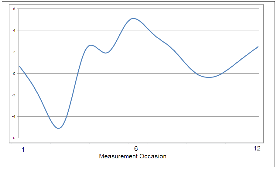
The approach introduced in this paper starts with fitting a growth model as defined in Equation (1) for each subject i and then uses the computed derivatives of each obtained natural cubic smooth spline function to algorithmically group or cluster individuals who follow the same growth trajectory patterns. For example, consider the following repeated measurements obtained from a single subject in a longitudinal study on event-based changes over time in infant looking behaviors (0.65, -2.57, -4.72, 2.14, 1.91, 4.92, 3.86, 2.27, 0.13, -0.25, 1.08, 2.60 - a similar developmental study was recently conducted by Yamashiro, Shrout, and Vouloumanos (2019). The measurements basically represent infant reaction time scores to initiate a gaze when observing an action. Figure 1 shows a plot of the natural cubic smoothing spline for this illustrative observation, and bears a clear nonlinear pattern of growth. Using the computerized implementation described and illustrated by Marcoulides and Khojasteh (2018), the second derivatives of the displayed cubic smoothing spline function are, 0, -3.10, 18.90, -18.34, 11.84, -9.59, 2.12, -2.04, 2.66, 1.96, -0.20, 0, respectively.3
It was noted previously that the second derivatives reflect the amount by which the slope is changing. This implies that if the function is very smooth then the derivative will take on a small value whereas major changes over time will result in large values. The second derivatives can also be used to answer the question of whether a particular score obtained at some measured time point is a minimum or a maximum (Borg & Groenen, 2005). Specifically, this implies that if, for some time point x the second derivative of the function \(f'' < 0\), then it is a maximum, whereas if \(f'' > 0\), then it is a minimum. As can be seen by examining the second derivatives for the examined illustrative infant looking behavior data given above, they signify multiple major changes are occurring over time, with the values being rather sizeable at time points 3 and 4. Although the usefulness of examining the derivatives of a growth curve as a way to assess the acceleration changes and the point in time when acceleration might reach a maximum or minimum value have been noted in the literature (Borg & Groenen, 2005; Marcoulides & Khojasteh, 2018; Suk, West, Fine, & Grimm, 2019, e.g.,), their consideration as tools for the clustering of individuals has not. As was also suggested by Liao (2005), we contend that in fact using these obtained parameter estimates of a growth model represents an ideal approach for the clustering of time-series data of any type. Data representation is without doubt one of the main challenging issues for any time-series clustering approach due in part to the multidimensional nature of the data. By utilizing derivatives of growth curves to group individuals who follow the same growth trajectory patterns, both local and global shape characteristics of the time series data are maintained in the obtained parameter estimates (Bagnall & Janacek, 2005; Liao, 2005). In this manner, even datasets exhibiting exceptionally complex growth patterns are not expected to impact the proposed clustering methodology (Giraud, 2022).
In order to determine groupings of individuals (should they exist), it is assumed that subjects in an observed sample belong to K different clusters or classes (G1, …., GK), such that individuals in each group have similar growth function derivatives. All natural cubic smooth spline functions and their derivatives are obtained separately for each examined individual with no assumptions regarding their distributions. Although it is possible to apply the approach to existing group level data (e.g., children assembled or grouped according to cognitive abilities), it is further assumed that all analyses will be conducted with data at the individual level. The algorithm then utilizes a closeness measure to evaluate the distance between observations and estimates the unknown number of classes with a hierarchical clustering algorithm via a threshold rule applied to the generated dendrogram. A dendrogram basically represents a tree-based taxonomy of the observations and is generally depicted as an upside-down tree built from leaves and branches (where each leaf represents a data point), and the combining or clustering of leaves and branches up to form the trunk (James et al., 2013). Hierarchical clustering is currently a very popular approach to group individual observations according to their degree of similarity or closeness. Hierarchical clustering can be thought of as a recursive partitioning of the data into successively smaller sets of observations based on their similarities4 . A major advantage of hierarchical clustering over other types of clustering approaches is that it does not require the number of groups (or their size) to be specified beforehand (Newman, 2004), but instead relies on the generated dendrogram to determine the appropriate partitioning of the data.
To apply the proposed clustering approach, it is further suggested that the similarity or closeness of individuals be determined using a derivative-based distance measure between the computed derivatives of each natural cubic smooth spline function. Various other forms of distance measures have also been suggested in the functional data analysis literature, although these generally do not focus on second-order derivatives and are therefore unable to measure the complete shape similarities or dissimilarities between examined functions (e.g., Ieva, Paganoni, Pigoli, & Vitelli, 2012; Tarpey & Kinateder, 2003). Specifically, we define a derivative-based distance measure between the computed derivatives for observations (say for i and j) over an entire time interval t as follows: \begin {equation} D(i,j) = \ \left \lbrack \int _{t}^{}\left \lbrack \left \lbrack f^{''}\left ( x_{i} \right ) - f^{''}\left ( x_{j} \right ) \right \rbrack ^{2}dt \right \rbrack \right \rbrack ^{\frac {1}{2}} \label {eq3} \end {equation} where \(D(i,j)\) is the distance measure, while \(f^{''}\left ( x_{i} \right )\) and \(f^{''}\left ( x_{j} \right )\) respectively denote the second derivatives of the functions for observations i and j. It is further assumed that \(D(i,j) \geq 0\), \(D(i,j) = \ D(j,i)\), and lastly that \(D(i,j) = 0\), if i = j. Thus, based on obtained distance measures of the derivatives for say observations i, j, and k using Equation (3), observation i would be declared to be more similar to observation j than to observation k if \(D(i,j) < D(i,k)\), where \(D(i,j)\ \)is the distance measure between individuals i and j and \(D(i,k)\ \)is the distance measure between individuals i and k. Upon computing all pairwise observations comparisons in the longitudinal data set, the derived distance matrix is then subjected to hierarchical clustering leading to similar observations being iteratively grouped together.
This section demonstrates the use of the proposed approach to determine groupings of individual observations in longitudinal data settings based on their computed growth function derivatives. For the purpose of this analysis, longitudinal data from 200 individuals from two distinct mixtures of complex autoregressive time series over 12 measurement occasions were simulated using the R function ‘arima.sim’ (with each cluster specified to contain an equal number of observations). This type of longitudinal growth model is very popular and commonly used for the study of inter-individual differences in intra-individual changes over time (Bulteel, Mestdagh, Tuerlinckx, & Ceulemans, 2018; Hamaker et al., 2018). The data and the parameters of the autoregressive times series were modeled following a detailed review of the literature on past growth mixture modeling empirical and simulation studies (e.g., He & Fan, 2019; Lubke & Muthén, 2005, 2007; Nylund, Asparouhov, & Muthén, 2007; Peugh & Fan, 2012; Wang & Bodner, 2007). Specifically, the data and their various complex growth patterns were modeled after the Berkeley Growth Study, which is a well-known study that traces the intellectual, motor, and physical development of infants (Bayley, 1933; Jones & Bayley, 1941). This data set often serves as a benchmark to test proposed clustering algorithm accuracy (Ramsay & Silverman, 2005). Previous analyses of empirical data of the cognitive scores of children on the California First-Year Mental Scale (CFYMS; administered as part of the Berkeley Growth Study every month from 1 to 12 months of age), were found to follow growth trajectory patterns that were characterized by sharp nonlinear changes in measured cognitive ability as the infants get older (Grimm & Marcoulides, 2016). These nonlinear changes provide a typical example of a longitudinal study where complex growth patterns are encountered.
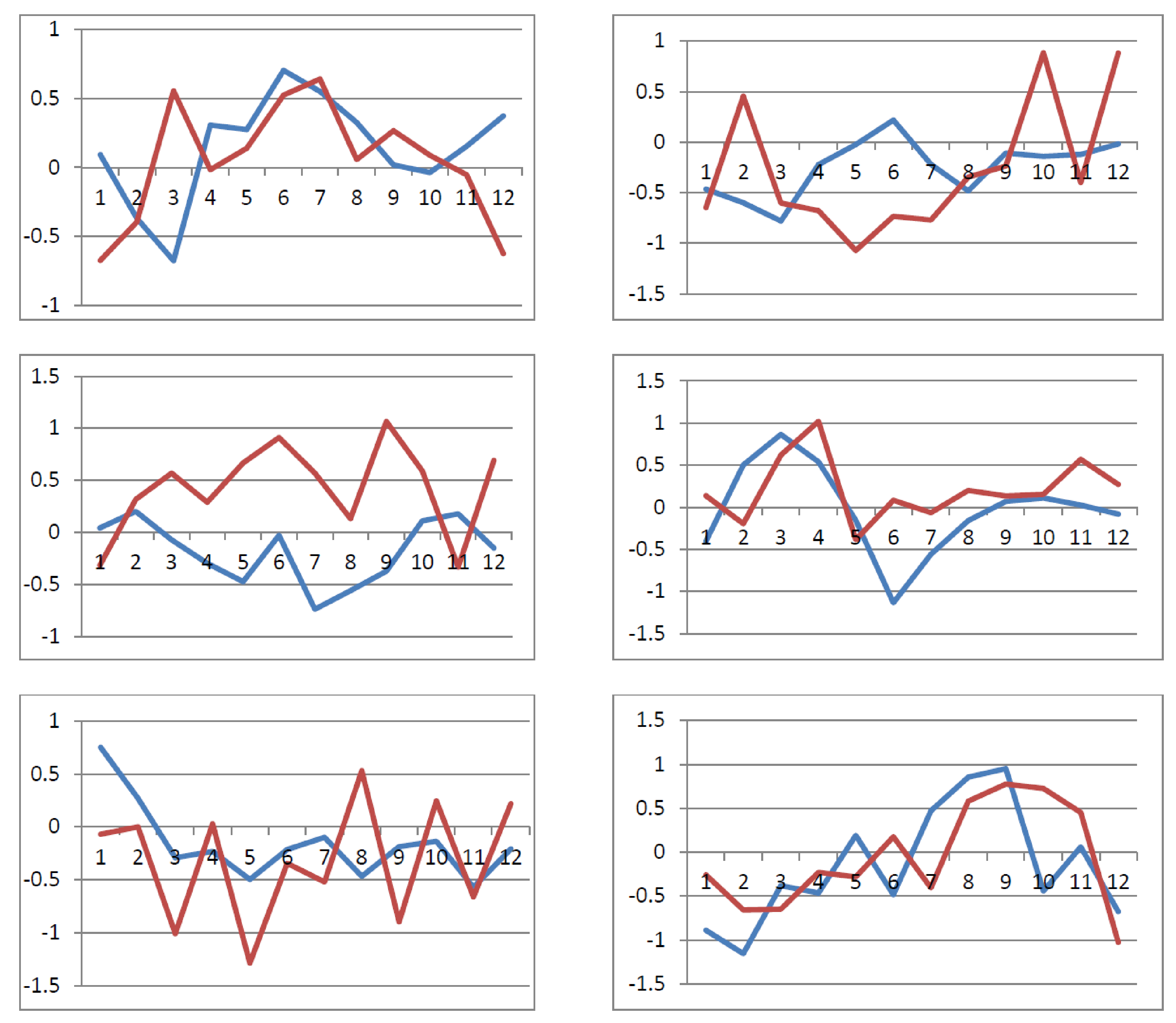
Consider for example the six complex times series trajectories displayed in Figure 2. Each panel presented in Figure 2 corresponds to the trajectories of two randomly generated individuals and are all characterized by nonlinear patterns of changes occurring over time. As can be seen by examining each of the presented panels in Figure 2, the six selected individuals in some instances display somewhat similar patterns of nonlinear changes and in other cases are markedly different. Although plots like these allow one with relative ease to graphically investigate whether individual growth trajectories differ from person to person, the benefit of the proposed approach is that it can algorithmically discern differences between individuals and determine those that belong together in a cluster based solely on their computed growth function derivatives.
To illustrate the comparison of individuals using their second derivatives, the observed scores for just three observations are considered next. It is important to note that in accordance with the model specification of their growth patterns, Person 1 and Person 3 are a priori specified as belonging to the same class, whereas Person 2 belongs to a different class. Figure 3 displays the individual cubic smoothing splines of these selected observations, and while some distinctions between the observations are evident, discerning how best to cluster them into groups is not directly evident. Computing the second derivatives of their growth functions (as presented in Table 1) and examining the distance measure between these derivatives among the pairs of individuals using Equation 3, it is determined that \(D(1,2) = \ 26.94\), \(D(1,3) = 8.11\), and \(D(2,3) = 20.83\) (where 1, 2, 3 are respectively used to denote each person examined). Based on the obtained distance measures, it is evident that Person 1 and Person 3 have similar growth trajectories (and would accordingly be assigned to the same cluster), while Person 2 has a dissimilar growth trajectory (and assigned to a different cluster). It is important to note that electing to compute Euclidean distances of the raw scores for these observations would result in approximately equal distance metrics between the three observations, and thereby make it much harder to accurately cluster them. Examining instead distance measures of derivatives makes the clustering much easier. Past research by Ramsay and Silverman (2005) has similarly shown that distance metrics based on smoothed time series data result in better data representations than distance metrics based on raw time series data. Other empirical comparisons of distance measures performed by Ding, Trajcevski, Scheuermann, Wang, and Keogh (2008) and Fulcher, Little, and Jones (2013) have also resulted in similar conclusions and provide additional motivation and support for the proposed clustering approach.
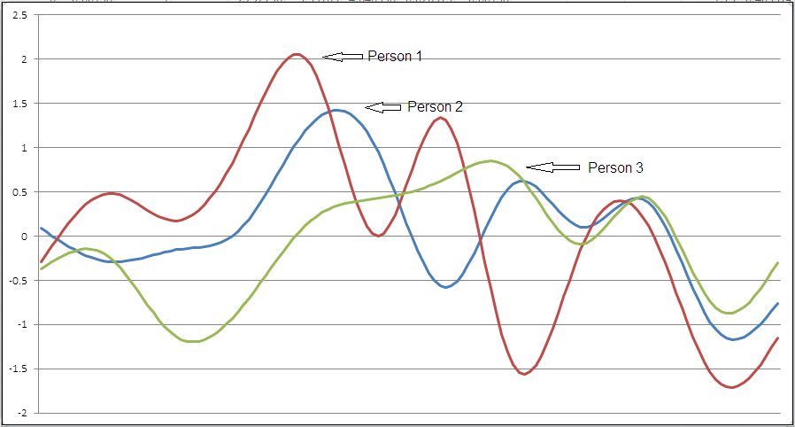
| Time Point | Person 1 | Person 2 | Person 3 |
| 1 | 0 | 0 | 0 |
| 2 | 0.904 | -2.143 | -2.123 |
| 3 | -0.507 | 2.073 | 2.242 |
| 4 | 1.933 | 1.116 | 0.672 |
| 5 | -1.962 | -6.798 | -1.275 |
| 6 | -2.846 | 9.292 | 0.185 |
| 7 | 5.999 | -10.853 | 0.365 |
| 8 | -4.87 | 9.606 | -2.431 |
| 9 | 3.473 | -3.119 | 3.783 |
| 10 | -4.397 | -3.316 | -4.561 |
| 11 | 3.821 | 4.299 | 3.909 |
| 12 | 0 | 0 | 0 |
Computing in the same manner the second derivatives of the growth functions for all 200 simulated individuals along with the distance measure between these derivatives and subjecting the obtained distance matrix among all pairs of individuals to a hierarchical clustering, would result in the dendrogram displayed in Figure 4. This dendrogram corresponds to a hierarchical cluster analysis of second derivatives on the complete simulated data for the 200 individuals a priori specified as belonging to two clusters. As can be seen, the two distinct mixtures of complex autoregressive time series over the measurement occasions are clearly visible and demonstrate the effectiveness of the proposed approach.

To investigate the estimation accuracy rates of the number of classes for the proposed approach, a small simulation study was conducted. Longitudinal data with distinct mixtures of autoregressive time series were simulated using the R function ‘arima.sim’. The proposed approach was implemented using the software program R (Marcoulides & Khojasteh, 2018; R Core Team, 2021) in combination with Microsoft Excel (via a programmed macro, data analysis tools, and spreadsheet template; see Marcoulides and Khojasteh (2018)).
Based on previous growth modeling studies in the literature, the number of time points and the degree of class separation were fixed in the simulation while the number of classes and sample size were varied (Nylund et al., 2007; Peugh & Fan, 2012). Specifically, the number of observed time points was set at t = 5, the degree of class separation (i.e., mean differences among clusters) was set at a value of 2 (to reflect moderately separated classes)5 , the number of true classes were set to range from 2 to 4 classes, and the sample sizes per class were set at N = 100, N = 500, and N = 1000 observations (to reflect small, medium, and large samples that were equally distributed across classes). Following the recommendations provided by a number of researchers (e.g., He & Fan, 2019; Kim, 2014; Nylund et al., 2007), a total of 100 replications were drawn for each model and time series condition. Correct estimation rates of the true number of classes we determined as the percentage of the total replications that were correctly identified (with high percentage values reflecting correctly identified number of classes; Nylund et al., 2007). It is important to note that because the proposed approach is algorithmically based, we do not compare its performance to traditional growth mixture modeling approaches. The determination of the number of classes in traditional approaches is based on a user subjectively applying various fit criteria (e.g., Nylund et al., 2007), thereby making the comparison between methods problematic and analogous to comparing the performance of an unsupervised data mining technique to a supervised technique – one is entirely algorithmically driven and the other involves user interface.
The correct estimation rates of the true number of classes are presented in Table 2. In summary, the simulation results clearly show the effectiveness of the proposed clustering method under a variety of examined conditions. As expected from past simulation studies in the growth mixture modeling literature, the overall performance accuracy of the approach was influenced by sample size (Nylund et al., 2007). For example, with small sample sizes per class (N = 100) the estimation rates were lower than when medium (N = 500) and large (N = 1000) sample sizes per class were analyzed. The influence of sample size on the estimation rates was present irrespective of the number of latent classes examined. Overall, the proposed approach showed consistently accurate estimation rates when the sample sizes were large (ranging from a low of 92% to a high of 98%), while with small sample sizes the estimation rates were slightly lower (ranging from a low of 88% to a high of 95%).
| Number of Classes | |||
| Sample Size | 2 | 3 | 4 |
| N = 100 | 0.908 | 0.879 | 0.955 |
| N = 500 | 0.922 | 0.968 | 0.964 |
| N = 1000 | 0.932 | 0.977 | 0.981 |
| Note. Sample size is per class.
| |||
Concluding Remarks
This article introduced a novel mixture modeling approach that can help researchers better understand patterns of growth trajectories and effectively be used to determine homogeneous and heterogeneous individual trajectories without imposing potentially problematic constraints on the model. The proposed approach can be considered as an unsupervised data-mining-oriented classification of individuals according to the derivatives of their estimated cubic smoothing spline functions. The proposed approach is ideally suited for fitting data in settings where normal mixtures might not be appropriate, particularly when assumptions regarding the trajectories are problematic (Genolini & Falissard, 2010; Usami, 2014). By utilizing a “bottom-up-approach” in which data are analyzed person by person, more insightful comparisons between the dynamics of different individuals could also be achieved. Not only does the proposed approach provide an ideal way to visualize complex growth data, but it can also be used to algorithmically reveal clustering of the growth patterns. The method can be used irrespective of the frequency of data collection or the complexity of the individual growth patterns, and provides an alternative lens through which dynamic processes can be examined.
A major problem with many of the highly popular procedures used in growth modeling is that they often impose overly restrictive assumptions on the model. In such instances, their effectiveness and accuracy are not always assured. The approach introduced in this paper is simply another alternative algorithmic-based modeling approach to help researchers examine and understand complex patterns of growth. Many options are available for the modeling of data from longitudinal studies and the approach introduced here represents a method to automate the determination of groupings of individuals (should they exist) entirely on the basis of their dynamic growth patterns utilizing cubic smoothing spline function derivatives.
Bagnall, A. J., & Janacek, G. (2005). Clustering time series with clipped data. Machine Learning, 58, 151–178. doi: https://doi.org/10.1007/s10994-005-5825-6
Baltes, P. B., & Nesselroade, J. R. (1979). Longitudinal research in the study of behavior and development. New York, NY: Academic Press.
Bayley, N. (1933). The California first-year mental scale (Vol. 243) [Computer software manual].
Bollen, K. A., & Curran, P. J. (2006). Latent curve models: A structural equation perspective. Hoboken, NJ: Wiley.
Borg, I., & Groenen, P. J. F. (2005). Modern multidimensional scaling: Theory and applications (2nd Ed). New York, NY: Springer.
Bulteel, K., Mestdagh, M., Tuerlinckx, F., & Ceulemans, E. (2018). Var(1) based models do not always outpredict AR(1) models in typical psychological applications. Psychological Methods, 23, 740–756. doi: https://doi.org/10.1037/met0000178
Diallo, T. M. O., Morin, A. J. S., & Lu, H. (2016). Impact of misspecifications of the latent variance-covariance and residual matrices on the class enumeration accuracy of growth mixture models. Structural Equation Modeling, 23. doi: https://doi.org/10.1080/10705511.2016.1169188
Ding, H., Trajcevski, G., Scheuermann, P., Wang, X., & Keogh, E. (2008). Querying and mining of time series data: Experimental comparison of representations and distance measures. Proceedings of the VLDB Endowment, 1(2). doi: https://doi.org/10.14778/1454159.1454226
Ezugwu, A. E., Ikotun, A. M., Oyelade, O. O., Abualigah, L., Agushaka, J. O., Eke, C. I., & Akinyelu, A. A. (2022, April). A comprehensive survey of clustering algorithms: State-of-the-art machine learning applications, taxonomy, challenges, and future research prospects. Engineering Applications of Artificial Intelligence, 110, 104743. doi: https://doi.org/10.1016/j.engappai.2022.104743
Finkel, D., Reynolds, C. A., McArdle, J. J., Gatz, M., & Pedersen, N. L. (2003). Latent growth curve analyses of accelerating decline in cognitive abilities in late adulthood. Developmental Psychology, 39, 535–550. doi: https://doi.org/10.1037/0012-1649.39.3.535
Flora, D. B. (2008). Specifying piecewise latent trajectory models for longitudinal data. Structural Equation Modeling, 15. doi: https://doi.org/10.1080/10705510802154349
Fraely, C., & Raftery, A. E. (1998). How many clusters? Which clustering method? Answers via model-based cluster analysis. The Computer Journal, 41, 578–588. doi: https://doi.org/10.1093/comjnl/41.8.578
Fulcher, B., Little, M., & Jones, N. (2013). Highly comparative time series analysis: The empirical structure of time series and their methods. Journal of the Royal Society Interface, 10(83), 20130048. doi: https://doi.org/10.1098/rsif.2013.0048
Gates, K. M., Lane, S. T., Varangis, E., Giovanello, K., & Guiskewicz, K. (2017). Unsupervised classification during time-series model building. Multivariate Behavioral Research, 52, 129–148. doi: https://doi.org/10.1080/00273171.2016.1256187
Genolini, C., & Falissard, B. (2010). Kml: K-means for longitudinal data. Computational Statistics, 25(2), 317–328. doi: https://doi.org/10.1007/s00180-009-0178-4
Gerald, C. F., & Wheatley, P. O. (2004). Applied numerical analysis (7th Ed.). Boston, MA: Pearson Education, Inc.
Giraud, C. (2022). Introduction to high-dimensional statistics. Chapman and Hall/CRC.
Green, P., & Silverman, B. (1994). Nonparametric regression and generalized linear models: A roughness penalty approach. Chapman & Hall/CRC Press, Boca Raton, FL. doi: https://doi.org/10.2307/1269920
Grimm, K. J., & Marcoulides, K. M. (2016). Individual change and the timing and onset of important life events: Methods, models, and assumptions. International Journal of Behavioral Development, 40, 87–96. doi: https://doi.org/10.1177/0165025415580806
Grimm, K. J., Ram, N., & Estabrook, R. (2016). Growth modeling: Structural equation and multilevel modeling approaches. New York, NY: Guilford Press.
Hamaker, E. L., Asparouhov, T., Brose, A., Schmiedek, F., & Muthén, B. (2018). At the frontiers of modeling intensive longitudinal data: Dynamic structural equation models for the affective measurements from the COGITO study. Multivariate Behavioral Research, 53, 820–841. doi: https://doi.org/10.1080/00273171.2018.1446819
Han, J., & Kamber, M. (2001). Data mining: Concepts and techniques. Waltham, MA: Morgan Kaufmann Publishers.
He, J., & Fan, X. (2019). Evaluating the performance of the k-fold cross-validation approach for model selection in growth mixture modeling. Structural Equation Modeling, 26. doi: https://doi.org/10.1080/10705511.2018.1500140
Hipp, J. R., & Bauer, D. J. (2006). Local solutions in the estimation of growth mixture models. Psychological Methods, 11, 36–53. doi: https://doi.org/10.1037/1082-989x.11.1.36
Ieva, F., Paganoni, A. M., Pigoli, D., & Vitelli, V. (2012). Multivariate functional clustering for the analysis of ECG curves morphology. Journal of the Royal Statistical Society. Series C. Applied Statistics, 62, 401–418. doi: https://doi.org/10.1111/j.1467-9876.2012.01062.x
Infurna, F. J., & Grimm, K. J. (2018). The use of growth mixture modeling for studying resilience to major life stressors in adulthood and old age: Lessons for class size and identification and model selection. Journal of Gerontology Series B: Psychological Sciences and Social Sciences, 73, 148–159. doi: https://doi.org/10.1093/geronb/gbx019
Infurna, F. J., & Luthar, S. S. (2016). Resilience to major life stressors is not as common as thought. Perspectives on Psychological Science, 11. doi: https://doi.org/10.1177/1745691615621271
James, G., Witten, D., Hastie, T., & Tibshirani, R. (2013). An introduction to statistical learning with applications in R. New York, NY: Springer. doi: https://doi.org/10.1007/978-1-0716-1418-1
Jones, H. E., & Bayley, N. (1941). The Berkeley growth study. Child Development, 12. doi: https://doi.org/10.2307/1125347
Kim, S.-Y. (2014, April). Determining the number of latent classes in single- and multiphase growth mixture models. Structural Equation Modeling: A Multidisciplinary Journal, 21(2), 263–279. doi: https://doi.org/10.1080/10705511.2014.882690
Liao, T. W. (2005). Clustering of time series data: A survey. Pattern Recognition, 38. doi: https://doi.org/10.1016/j.patcog.2005.01.025
Lin, X., & Zhang, D. (1999). Inference in generalized additive mixed model using smoothing splines. Journal of the Royal Statistical Society, Series B, 61. doi: https://doi.org/10.1111/1467-9868.00183
Lubke, G. H., & Muthén, B. O. (2005). Investigating population heterogeneity with factor mixture models. Psychological Methods, 10, 21–39. doi: https://doi.org/10.1037/1082-989x.10.1.21
Lubke, G. H., & Muthén, B. O. (2007). Performance of factor mixture models as a function of model size, covariate effects, and class-specific parameters. Structural Equation Modeling, 14, 26–47. doi: https://doi.org/10.1080/10705510709336735
Marcoulides, K. M. (2018). Automated latent growth curve model fitting: A segmentation and knot selection approach. Structural Equation Modeling, 25, 687–699. doi: https://doi.org/10.1080/10705511.2018.1424548
Marcoulides, K. M., & Khojasteh, J. (2018). Analyzing longitudinal data using natural cubic smoothing splines. Structural Equation Modeling, 25, 965–971. doi: https://doi.org/10.1080/10705511.2018.1449113
Marcoulides, K. M., & Trinchera, L. (2019). Detecting unobserved heterogeneity in latent growth curve models. Structural Equation Modeling, 26, 390–401. doi: https://doi.org/10.1080/10705511.2018.1534591
Marcoulides, K. M., & Trinchera, L. (2021, February). Residual-based algorithm for growth mixture modeling: A monte carlo simulation study. Frontiers in Psychology, 12. doi: https://doi.org/10.3389/fpsyg.2021.618647
McArdle, J. J., & Nesselroade, J. R. (2014). Longitudinal data analysis using structural equation models. Washington, DC: American Psychological Association. doi: https://doi.org/10.1037/14440-000
Muthén, B. O. (2001). Latent variable mixture modeling. In G. A. Marcoulides & R. E. Schumacker (Eds.), New developments and techniques in structural equation modeling (pp. 1–33). Mahwah, NJ: Lawrence Erlbaum Associates.
Muthén, B. O., & Shedden, K. (1999). Finite mixture modeling with mixture outcomes using the EM algorithm. Biometrics, 55. doi: https://doi.org/10.1111/j.0006-341x.1999.00463.x
Nagin, D. S. (2005). Group-based modeling of development. Cambridge, MA: Harvard University Press. doi: https://doi.org/10.4159/9780674041318
Newman, M. E. (2004). Detecting community structure in networks. European Physical Journal B, 38, 321–330. doi: https://doi.org/10.1140/epjb/e2004-00124-y
Nylund, K. L., Asparouhov, T., & Muthén, B. O. (2007). Deciding on the number of classes in latent class analysis and growth mixture modeling: A Monte Carlo simulation study. Structural Equation Modeling, 14, 535–569. doi: https://doi.org/10.1080/10705510701575396
Peugh, J., & Fan, X. (2012). How well does growth mixture modeling identify heterogeneous growth trajectories? A simulation study examining GMM’s performance characteristics. Structural Equation Modeling, 19, 204–226. doi: https://doi.org/10.1080/10705511.2012.659618
R Core Team. (2021). R: A language and environment for statistical computing [Computer software manual]. Vienna, Austria. Retrieved from https://www.R-project.org/
Ramsay, J. O., & Silverman, B. W. (2005). Functional data analysis (2nd Ed.). New York, NY: Springer-Verlag.
Rice, J. R. (1976). Adaptive approximation. Approximation Theory, 16, 239–337. doi: https://doi.org/10.1016/0021-9045(76)90065-4
Ruscio, J. (2007). Taxometric analysis: An empirically grounded approach to implementing the method. Criminal Justice and Behavior, 34, 1588–1622. doi: https://doi.org/10.1177/0093854807307027
Suk, H. W., West, S. G., Fine, K. L., & Grimm, K. J. (2019). Nonlinear growth curve modeling using penalized spline models: A gentle introduction. Psychological Methods, 24(3), 269–290. doi: https://doi.org/10.1037/met0000193
Tarpey, T., & Kinateder, K. K. J. (2003). Clustering functional data. Journal of Classification, 20, 93–114. doi: https://doi.org/10.1007/s00357-003-0007-3
Usami, S. (2014). Constrained k-means on cluster proportion and distances among clusters for longitudinal data analysis. Japanese Psychological Research, 56(4), 361–372. doi: https://doi.org/10.1111/jpr.12060
Wang, M., & Bodner, T. E. (2007). Growth mixture modeling: Identifying and predicting unobserved subpopulations with longitudinal data. Organizational Research Methods, 10, 635–656. doi: https://doi.org/10.1177/1094428106289397
Wood, P. K., Steinley, D., & Jackson, K. M. (2015). Right-sizing statistical models for longitudinal data. Psychological Methods, 20, 470–488. doi: https://doi.org/10.1037/met0000037
Yamashiro, A., Shrout, P. E., & Vouloumanos, A. (2019). Using spline models to analyze event-based changes in eye tracking data. Journal of Cognition and Development, 20, 299–313. doi: https://doi.org/10.1080/15248372.2019.1583231