Keywords: Bayesian Growth Curve Modeling · Random Slope Testing · Longitudinal Data Analysis · Permutation Testing.
Longitudinal research design is a powerful framework for testing psychological hypotheses regarding change. In such a framework, researchers measure the same construct from multiple participants across multiple time points so as to study how a given psychological process changes over time (Baltes & Nesselroade, 1979). Due to the versatility and statistical power afforded by longitudinal research designs, researchers have been able to study time-varying phenomena such as patterns and outcomes of drug use among adolescents, trajectories of public reaction to large-scale disasters, and stability of personality traits across time (Roberts, Walton, & Viechtbauer, 2006; Shedler & Block, 1990; Silver, Holman, McIntosh, Poulin, & Gil-Rivas, 2002). By collecting data in a longitudinal manner, researchers are able to simultaneously study how a given psychological construct changes within an individual and what factors influence the varying trajectories of said construct among different individuals.
Although collecting data in a longitudinal manner may be more difficult than collecting data in a single wave, advances in data collection technologies have made longitudinal research designs accessible to many researchers. As such, in recent years longitudinal research designs have become commonplace in psychological research. A Google Scholar search for the terms “longitudinal”, “research”, and “psychology” shows an increase in number of related works from about 140,000 results in the 1990s to more than 1,200,000 related works between 2010 and 2020. With this increase in popularity of longitudinal research designs there has also come an increase in the number and quality of statistical methods for analysing longitudinal data. Although varied, each method provides researchers some insight into how psychological processes change over time.
Statistical methods for longitudinal data analysis help researchers to understand both intraindividual change and interindividual differences in intraindividual change across time. That is, researchers may use statistical methods for longitudinal data analysis in order to gain a deeper understanding of how individuals change over time with respect to a variable of interest and how different individuals may show different patterns of change. Growth curves modeling is one popular way of assessing these qualities given a longitudinal sample of participants (Grimm, Ram, & Estabrook, 2016; Hertzog & Nesselroade, 2003; Oravecz & Muth, 2018). Growth curve models have been used by researchers to study a wide variety of phenomena such as academic trajectories of children, the development of individuals’ self-esteem, and changes in depressive symptoms of adolescents over time (Baldwin & Hoffmann, 2002; Gomez-Baya, Mendoza, Paino, Sanchez, & Romero, 2016; Gutman, Sameroff, & Cole, 2003). Due to the simplicity and flexibility of growth curve models, different researchers may use different statistical frameworks for estimating growth curve models. Such statistical frameworks for conducting growth curve analyses include mixed-effects modeling/multilevel modeling and structural equation modeling.
Across statistical frameworks, growth curve models generally take the form: \begin {equation} Y_{ij}=\beta _{0}+\beta _1T_j+u_{0i}+u_{1i}T_j+\epsilon _{ij}, \label {GC} \end {equation} where \(Y_{ij}\) is the realizatio of an outcome variable from person i at time j, \(i=1,\ldots ,N\), \(j=1,\ldots ,K\), where N is the sample size and K is the total number of measurement occasions, \(\beta _0\) is a fixed effect representing the average intercept value at time \(T_j=0\) for all participants, \(\beta _1\) is a fixed effect representing the average slope over time, \(u_{0i}\) is a random component of intercept for each individual \(i\) with variance \(\sigma ^2_{u_{0}}\), at time \(T_j=0\), \(u_{1i}\) is a random component of slope for each individual \(i\) with variance \(\sigma ^2_{u_{1}}\), and \(\epsilon \) is an error term with variance \(\sigma ^2_{\epsilon }\). Specific and meaningful interpretation of these parameters have allowed for growth curve modeling to become a common tool for studying change (McArdle & Nesselroade, 2003). Fixed-effect parameters relate to general trends across all participants, while random-effect parameters relate to individual participant variation from this overall group level behavior. Multiple statistical software packages are capable of estimating parameters of growth curve models using various techniques.
Bayesian analysis is one way of estimating growth curve models for a given longitudinal data set (Fearn, 1975; Oravecz & Muth, 2018; Zhang, Hamagami, Wang, Nesselroade, & Grimm, 2007). Compared to other analysis frameworks, Bayesian analysis allows researchers a high degree of flexibility in modeling complex longitudinal patterns of change. While many modern analysis methods have strict assumptions of normality and other asymptotic assumptions, researchers using Bayesian analyses are generally not limited by these concerns asprior distributions of all variables can be explicitly and flexibly modeled (Bayarri & Berger, 2004). Thus common longitudinal data analysis problems such as sample size restrictions, non-normal data distributions, and missing data patterns due to attrition are more easily handled in a Bayesian framework than in a frequentist framework. Additionally, advancement in computational efficiency and Bayesian analysis software has helped ease the burden of conducting Bayesian analysis put on researchers new to Bayesian modeling (e.g., JAGS, STAN, BUGS).
In a Bayesian framework, parameters of a growth curve model are treated as random variables whose realizations are modeled using some form of a Markov chain Monte Carlo (MCMC) process such as Gibbs sampling to sample from constantly updated distributions (Carlin & Chib, 1995; Gilks, Wang, Yvonnet, & Coursaget, 1993). Equation (1) can also be expressed as: \begin {equation} \begin {split} Y_{ij}\sim N(\bar {Y}_{ij},\sigma ^2_{\epsilon })\\ \bar {Y}_{ij}=b_{0i}+b_{1i}T_j\\ b_{0i}\sim N(\beta _{0},\sigma ^2_{u_{0}})\\ b_{1i}\sim N(\beta _{1},\sigma ^2_{u_{1}}), \label {BGC} \end {split} \end {equation} where \(\bar {Y}_{ij}\) is the expected value of \(Y_{ij}\). This Bayesian parameterization of a growth curve model allows researchers to use previous knowledge to hypothesize the prior distributions of the parameters \(\beta _{0}, \beta _{1}, \sigma ^2_{u_{0}}, \sigma ^2_{u_{1}}\), and \(\sigma ^2_{\epsilon }\). Parameters \(b_{0i}\) and \(b_{1i}\) may also be correlated. In such a case an additional parameter, \(\sigma _{u_{0}u_{1}}\), is also modeled. Typically researchers set priors for \(\beta _{0}\) and \(\beta _{1}\) as either normal or uniform distributions, while setting priors of the variance components \(\sigma ^2_{u_{0}}\), \(\sigma ^2_{u_{1}}\), and \(\sigma ^2_{\epsilon }\) as inverse gamma distributions, although other distributions have been assessed (Gelman, 2006; Zhang, 2016; Zhang et al., 2007). These priors are then iteratively updated into posterior distributions using data. After a large number of iterations, a Bayesian model will converge, parameter estimates will remain stable, and researchers may draw statistical inference.
Substantive researchers routinely need to determine the statistical significance of each parameter. Credible intervals are a commonly used in Bayesian growth curve modeling (Zhang et al., 2007). A \(100\times (1-\alpha )\%\) credible interval for a parameter is as an interval for which there is at least a \(100\times (1-\alpha )\%\) chance said interval contains the true value of a given parameter, conditional on a given data set. Similar to a frequentist confidence interval, a parameter is considered significant at the \(\alpha \)-level when a \(100\times (1-\alpha )\%\) credible interval for said parameter does not include 0. While versatile, credible intervals are not useful for testing variance components of Bayesian growth curves. This is because the gamma/inverse gamma distributions used to model such variance components are bounded \((0,\infty )\). Also, parameters with gamma/inverse gamma distributed priors tend to also have gamma/inverse gamma distributed posteriors. In such a case, a Bayesian credible interval at any \(\alpha \)-level will never include a 0 value (Gelman, 2006). This boundary problem makes Bayesian hypothesis testing using credible intervals completely ineffective for testing variance parameters, thus making statistical inference on the existence of significant individual differences in interindividual change impossible. Fortunately, there are ways to overcome this problem. In this article, we review alternative methods to credibility intervals for testing for the existence of interindividual differences in intraindividual change in growth curve models and propose a new test based upon data permutations.
This problem of determining the existence of interindividual differences in intraindividual change can be viewed as a problem of model comparison and selection. That is, determining if a model which includes a parameter indicative of interindividual differences in intraindividual change fits data better than a model without such a parameter. In determining how to specify such a model, Barr, Levy, Scheepers, and Tily (2013) argued for using the most complex structure admissible for a given data set; see also Barr (2013). Other researchers such as Bates, Kliegl, Vasishth, and Baayen (2015) and Matuschek, Kliegl, Vasishth, Baayen, and Bates (2017), urged caution when using such an approach as more complex models may lead to convergence issues, as well as a a loss of statistical power. Model selection is key for accurately assessing all important effects, while minimizing estimation issues. Many methods currently exist for testing for significant random slope parameters within a frequentist framework by determining an optimal model structure. These include likelihood based comparison methods, penalty functions, and information criterion (Fan & Li, 2012; Peng & Lu, 2012; Stram & Lee, 1994; Vaida & Blanchard, 2005). There are currently fewer methods for testing for significant random slope paramters within a Bayesian growth curve context. Perhaps the most common methods for Bayesian model comparison are using deviance information criterion (DIC) values and Bayes factors.
Deviance information criterion is an information metric derived from the posterior distribution of the log-likelihood of a given data set and a penalization value based on the complexity of a given model (Spiegelhalter, Best, & Carlin, 1998; Spiegelhalter, Best, Carlin, & van der Linde, 2002). DIC is calculated as: \begin {equation} \begin {split} DIC=E_{\theta |y}[D(\theta )]+p_D\\ D(\theta )=-2log(L(\theta |y))\\ p_D=E_{\theta |y}[D(\theta )]-D(E_{\theta |y}[\theta ]), \label {DIC} \end {split} \end {equation} where \(\theta \) is the parameterization of a given model, \(L(\theta |y)\) is the likelihood of \(\theta \) given some data, \(y\), \(E_{\theta |y}[D(\theta )]\) is a the expectation of \(D(\theta )\) conditional on \(y\), and \(E_{\theta |y}[\theta ]\) is the expectation of \(\theta \) conditional on \(y\).
As a model’s likelihood increases, \(D(\theta )\) tends to \(0\). Conversely, as the number of parameters in a model increase, so does \(p_D\). In this way DIC simultaneously incorporates model fit and penalizes overly complex models. For model comparison purposes on a given data set, model selection by DIC is conducted by selecting the model with a lower DIC value by at least 10 points, otherwise selecting the model with fewer parameters (Spiegelhalter et al., 1998). Thus, a researcher interested in testing for the existence of interindividual differences in intraindividual change across time within his/her own data would compare the DIC values of two competing growth cruve models. One model would allow the slope parameter to vary by participant, and another model would fix this value to be the same for all participants. Assuming a DIC difference of more than 10 points, the model with a lower DIC value would then be considered more appropriate for these data than the model with a higher DIC value (Lunn, Jackson, Best, Spiegelhalter, & Thomas, 2012).
Although DIC is a relatively reliable metric for model selection it is not without its criticisms. According to a review by Spiegelhalter et al. (2014), some of the most common criticisms of DIC is its lack of consistency and its weak theoretical justification. As an alternative to model comparison using DIC, some researchers argue for the use of Bayes factors (Ward, 2008).
The Bayes factor is another common measure for model comparison within a Bayesian framework (Kass & Raftery, 1995; Lodewyckx et al., 2011; Saville & Herring, 2009). Bayes factors can be thought of as a ratio of evidence for one model over another, which is evident in its calculation: \begin {equation} B=\frac {p(y|M_1)}{p(y|M_2)}=\frac {p(M_1|y)}{p(M_2|y)}\frac {p(M_2)}{p(M_1)}, \label {BF} \end {equation} where \(M_1\) and \(M_2\) are different models used on the same data, \(y\). The Bayes factor, \(B\), can then be used for model selection. For \(B > 3\), one would say that there is substantial evidence for \(M_2\) over \(M_1\) and thus a researcher would select \(M_2\) as the more probable model. If however \(B < \frac {1}{3}\), a researcher would select \(M_1\) as the more probable model for the generation of \(y\) (Stefan, Gronau, Schönbrodt, & Wagenmakers, 2019).
Although intuitive, Bayes factors can be difficult to obtain analytically and calculations for their numeric approximations can be computationally intensive for some models or require hyper-parameters to be set by a researcher. Additionally there are methods for numerically approximating Bayes factors including so called default Bayes factors, approximate Bayes factors, and Bayes factors estimated through the product space method (Lodewyckx et al., 2011; Rouder & Morey, 2012; Saville & Herring, 2009). Each of these methods for estimating Bayes factors require time and energy for a researcher to understand each method’s intricacies well enough to properly implement each method. Bayes factor calculations may also be sensitive to a researcher’s specification of priors (Ward, 2008). Additionally, implementations of Bayes factors have been shown to be inappropriate for many data sources and Bayes factors themselves have been argued as having frequentist properties, making many numerically approximated Bayes factors uninformative (Hoijtink, van Kooten, & Hulsker, 2016; Morey, Wagenmakers, & Rouder, 2016). Such difficulties make estimation of Bayes factors using for more complex models, such as growth curves, intractable. Indeed the authors of this article could find no reliable method for estimating Bayes factors for growth curve models as most numerical methods are either not able to take into account random effect structures or require overly sensitive hyper-parameter settings to initiate jumping behaviors between models needed to obtain proper Bayes factor approximations (Lodewyckx et al., 2011; Rouder & Morey, 2012; Saville & Herring, 2009). Many current methods that do offer Bayes factors for random effects models do not give Bayes factor values for the random effects parameters of interest in this aritcle. Thus, a researcher would find difficulty in using Bayes factors for testing for the existence of interindividual differences in intraindividual change across time. Although the DIC and Bayes factor methods are not the only methods used to assesses the random effects structure of growth models, these are perhaps the most common (Cai & Dunson, 2006; Chen & Dunson, 2003; Piironen & Vehtari, 2017; Ward, 2008).
The DIC and Bayes factor methods share a common quality, each are model driven approaches. With either method, a researcher must specify two separate models that are then compared to one another. Thus, in order to test for the existence of a quality of interest within a data set, the models themselves are modified and the associated data are left alone. In contrast, data driven methods such as bootstrap analyses, randomization tests, and surrogate data analyses have been shown to also be effective at establishing existence of a specific quality of interest within a given data set (Efron, 1979; Moulder, Boker, Ramseyer, & Tschacher, 2018; Theiler, Eubank, Longtin, Galdrikian, & Farmer, 1992). These methods rely on modifying data sets through some randomized approach such as sampling with replacement or data shuffling, to destroy qualities of order and structure within a given data set.
With this in mind, we propose a simple and relatively uncomplicated data driven method for determining the existence of interindividual differences in intraindividual change in a Bayesian growth curve framework. Namely, we propose a data permutation algorithm which effectively tests if a random slope parameter is reliably distinguishable from random noise. In terms of model selection, this would be similar to determining if the model in Equation (2) fits the data better than a simpler model with a fixed slope: \begin {equation} \begin {split} Y_{ij}\sim N(\bar {Y}_{ij},\sigma ^2_{\epsilon }),\\ \bar {Y}_{ij}=b_{0i}+\beta _1T_j,\\ b_{0i}\sim N(\beta _{0},\sigma ^2_{u_{0}}). \label {BGCSlope} \end {split} \end {equation}
Our proposed data permutation algorithm is as follows:
Create a fully specified Bayesian growth curve model (Equation 2) including a random slope term, using unaltered/original data, denoted as \(y_0\), and store the posterior samples of \(\sigma ^2_{u_{1}}|y_0\) obtained from a MCMC procedure after a burn-in period.
Consistently sort data either descending or ascending at each time point to create a second data set, \(y_{sort}\).
Rerun step i) using \(y_{sort}\), and store the samples of \(\sigma ^2_{u_{1}}|y_{sort}\).
Randomly shuffle \(y_0\) within each time point to create a third data set, \(y_{shuff}\).
Rerun step i) using \(y_{shuff}\), and store the samples of \(\sigma ^2_{u_{1}}|y_{shuff}\).
Compare the mean of the samples from \(\sigma ^2_{u_{1i}}|y_0\), \(\mu _0\), with the mean of the samples of \(\sigma ^2_{u_{1}}|y_{sort}\), \(\mu _{sort}\), and the mean of samples of \(\sigma ^2_{u_{1}}|y_{shuff}\), \(\mu _{shuff}\). If \(|\mu _0-\mu _{sort}|<|\mu _0-\mu _{shuff}|\) then slope term of the model can be said to reliably vary between individuals. Else the slope term can not reliably be said to vary between participants.
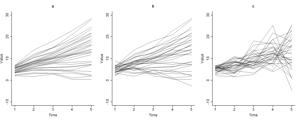
To understand how this algorithm works, consider Figure 1. Across all three plots, the parameters \(\beta _0\) (fixed intercept) and \(\beta _1\) (fixed slope) from equation (2) are all the same. Figure 1(b) represents the kind of data one might expect to find from a given research study, with \(\sigma ^2_{u_{0}}\), \(\sigma ^2_{u_{1}}\), and \(\sigma ^2_{\epsilon }\) all greater than 0. We will consider this data as \(y_0\) for this example. Figure 1(a) is the sorted version of \(y_0\), which we call \(y_{sort}\). Notice a few interesting qualities of \(y_{sort}\). Firstly, no line of \(y_{sort}\) crosses another. Also, the error variance about each individually modeled line is minimized. Thus the ratio of \(\sigma ^2_{u_{1i}}\) to \(\sigma ^2_{\epsilon _{ij}}\) for \(y_{sort}\) is larger than the same ratio for \(y_0\), assuming \(y_0\) is not already in a sorted state. The opposite is true for \(y_{shuff}\). Assuming that \(y_0\) had some intrinsic structure to itself due to some true and natural underlying growth phenomenon, the ratio of \(\sigma ^2_{u_{1}}\) to \(\sigma ^2_{\epsilon }\) for \(y_{shuff}\) should be smaller smaller than the same ratio for \(y_0\), Figure 1(c). The difference between the means of the posterior sampling distributions of \(p(\sigma ^2_{u_{1}}|y_{sort})\), \(p(\sigma ^2_{u_{1}}|y_0)\), and \(p(\sigma ^2_{u_{1}}|y_{shuff})\) then give a measure of how similar the three distributions of \(p(\sigma ^2_{u_{1}}|y)\) are. Thus if \(|\mu _0-\mu _{sort}|<|\mu _0-\mu _{shuff}|\), then the sampling distribution of the posterior distribution of \(\sigma ^2_{u_{1}}\) for the unedited data is more like the posterior distribution of \(\sigma ^2_{u_{1}}\) for data which has noticeable slope variation. If \(|\mu _0-\mu _{sort}|>|\mu _0-\mu _{shuff}|\), then the sampling distribution of the posterior distribution of \(\sigma ^2_{u_{1}}\) for the unedited data is more like the posterior distribution of \(\sigma ^2_{u_{1}}\) for data which has been randomly shuffled and has slope variation that is difficult to distinguish from random noise.
This method may be considered a form of a permutation test. Permutation tests are a class of tests for comparing a given test statistic to a distribution of these test statistics obtained from a random ordering of the data (Collingridge, 2013; Golland & Fischl, 2003; Pesarin & Salmaso, 2010; Theiler et al., 1992). This random ordering builds a test statistic under the distribution of a null-hypothesis that there is no natural order to the data. Any test statistic outside of a set \(\alpha \)-level, based on the permutation distribution, is then considered to be highly unlikely given random chance and thus must contain some meaningful and non-random structure. Our method differs from traditional permutation methods in that we propose the use of only a single random shuffle. This is because of the bounds set by 0 and \(\sigma ^2_{u_{1}}\) for \(y_{sort}\). Over multiple different parameterizations, we found that on a scale of 0 to \(\sigma ^2_{u_{1}}\) for \(y_{sort}\), the distribution of multiple random \(y_{shuff}\) is small in comparison (\(<5\%\) of the overall space). As such, one random shuffle should give a good approximation of the distribution of multiple random \(y_{shuff}\). However, should a researcher need more precision, taking an average of multiple random \(y_{shuff}\) values will give a more accurate result.
In order to gain an intuitive understanding of this algorithm, consider this analogy of an individual with messy hair who wants a new hair style from a barber. A customer (data) with messy hair walks into a barber shop and asks the barber (researcher) for a haircut fitting for said customer’s natural hair style. The barber accepts this request and beings work, but is unable to visually determine if the customer has naturally curly hair (variable slopes) or naturally straight hair (constant slopes) due to the current messy state of the customer’s hair. The barber knows however, that a natural property of hair is that curly hair is naturally difficult to straighten and straight hair is naturally difficult to curl. So the barber first attempts to straighten (sort) the customer’s hair and finds that the hair changed very little. The barber then attempts to curl (shuffle) the customer’s hair and finds the customer’s hair curled with ease and had changed much from its original messy state. Thus, the barber concludes that the customer had naturally curly hair as the messy state of the customer’s hair was most easily and most dramatically changed by curling (i.e., a reliable variation in slopes was found because \(|\mu _0-\mu _{sort}|<|\mu _0-\mu _{shuff}|\)).
The remainder of this article is structured as follows: First, a simulation is presented of the proposed permutation method compared to using DIC values for determining the existence of slope variation. Then an application of this method to data from the National Longitudinal Study of Adolescent to Adult Health is presented. Finally this article concludes with a discussion regarding the proposed method’s usefulness, an introduction to an analysis tool which facilitates the application of this method, limitations, and future directions.
In order to determine the effectiveness of the proposed data permutation method and to compare our method with a common model comparison procedure (i.e., DIC), a simulation study was conducted using the R programming language and OpenBUGS (Lunn, Spiegelhalter, Thomas, & Best, 2009; R Core Team, 2013). Each simulation generated data from one of two models: model A or model B. Data simulated from models A and B were also used to study the effectiveness of DIC values relative to the proposed data permutation method.
Model A is a model including a random slope term and is parameterized as: \begin {equation*} Y_{ij}=5+2T_j+u_{0i}+u_{1i}T_j+\epsilon _{ij}, \label {SimModA} \end {equation*} \begin {equation*} u_{0i} \sim Gaussian(0,1), \end {equation*} \begin {equation*} u_{1i} \sim Gaussian(0,\sigma ^2_{u_{1}}), \end {equation*} \begin {equation*} Cov(u_{0i},u_{1i},\epsilon _{ij})= \begin {bmatrix} 1 & 0 & 0 \\ 0 & \sigma ^2_{u_{1}} & 0 \\ 0 & 0 & 1 \end {bmatrix}. \end {equation*} Parameter values of 5 and 2 for \(\beta _0\) and \(\beta _1\), respectively, and \(T_j=j-1, j=1,\ldots ,5\) were chosen as simple examples of positive linear growth. The variance of parameter \(u_{0i}\) was set to 1 for all simulated data sets. As the proposed permutation method is a test of random slopes and not random intercepts, the variance of parameter \(u_{0i}\) is arbitrary. The covariance between parameters \(u_{0i}\) and \(u_{1i}\) was set to 0 as any covariance between \(u_{0i}\) and \(u_{1i}\) would necessitate variance of \(u_{1i}\), thus increasing the effectiveness of the proposed permutation method3 . The variance of the error term was held constant at 1 across all time points (Grimm & Widaman, 2010). Finally \(\sigma ^2_{u_{1}}\) was varied across simulations, \(\sigma ^2_{u_1}=.1, .2, \ldots , 2\). Model B is simply model A without a random slope term where \(u_{1i}=0\): \begin {equation*} Y_{ij}=5+2T_j+u_{0i}+\epsilon _{ij}, \label {SimModB} \end {equation*} \begin {equation*} u_{0i} \sim Gaussian(0,1), \end {equation*} \begin {equation*} u_{1i} \sim Gaussian(0,\sigma ^2_{u_{1}}), \end {equation*} \begin {equation*} Cov(u_{0i},\epsilon _{ij})= \begin {bmatrix} 1 & 0 \\ 0 & 1 \end {bmatrix}. \end {equation*} For data generated from model A and B, \(\sigma ^2_{u_{1}}\in [0,.1,.2,\ldots ,2]\). This creates \(\sigma ^2_{u_{1}}\) (signal) to \(\sigma ^2_{\epsilon }\) (noise) ratios ranging between 0% and 200% across both models A and B. Thus, in total 21 data generating models were used.
The choice of specific values for this simulation are mostly arbitrary as \(u_{1}\) is independent from \(\beta _0\) and \(\beta _1\), \(u_{0}\), and \(\epsilon _{ij}\). Thus any value choices for these terms should have no effect on the validity of this method as the proposed method is a comparison of only the similarity of \(\sigma ^2_{u_{1}}\) estimated from the observed data to only \(\sigma ^2_{u_{1}}\) of the same data organized in such a way that minimizes \(\sigma ^2_{\epsilon }\) versus the same data organized in a way to increase \(\sigma ^2_{\epsilon }\). Theoretically no other parameter values should influence our proposed method in the case that there is no covariance between random intercept and random slope terms.
For each round of simulation, \(N \in [50,200,500]\) individuals data were simulated from each of the 21 data generating models, \(\sigma ^2_{u_{1}}\in [0,.1,\ldots ,2]\). Each round of simulation generated 1,000 instances giving a total of 63,000 (3 x 21 x 1000) data sets. Using Equation (2), Bayesian growth curves were fit to data generated by models A and B. Model A represents data which has individual slope variation and thus can be used to compute statistical power and type-II error rates. Similarly, model B represents data with no individual slope variation and thus can be used to compute specificity and type-I error rates4 . Using DIC and the proposed data permutation method, guesses were made at each simulation step to determine if data were simulated from a process with fixed slope growth trajectory across individuals or with a growth trajectory whose slope varied per individual. These guesses were compared to known random effect structures to determine statistical power and specificity rates. Each model was run with 20,000 MCMC iterations and a burn-in period of 15,000 iterations using OpenBUGS and the R2OpenBUGS package in R (Lunn et al., 2009; Sturtz, Ligges, & Gelman, 2005). All models were checked for convergence with a Kolmogorov-Smirnov test (Brooks, Giudici, & Philippe, 2003). To ensure this method was not statistical package specific, we ran a similar simulation study using the MCMCglmm R package and found identical results (Hadfield, 2010).
For DIC comparison, two models were conducted at each simulation, one with a fixed slope growth trajectory across individuals and one with a growth trajectory whose slope varied per individual. If the model with a growth trajectory whose slope varied per individual had a DIC value 10 points lower than the model with a constant rate of change, data from this simulation were considered to have a growth trajectory whose slope varied per individual. Otherwise the simulated data for said simulation were considered to have a trajectory with constant rate of change across individuals. We compared two criterion for DIC selection: DIC \(>\) 10 and minimum DIC value(Spiegelhalter et al., 1998).
For data permutation comparison, at each simulation step a model with a growth trajectory whose slope varied per individual was run on the data for that simulation step and the average value of \(\sigma ^2_{u_{1}}\) was recorded. Data was then sorted by column in descending order and a second model was run on the sorted data, storing \(\sigma ^2_{u_{1}}\) for this model. Finally data were randomly shuffled per column and a third model was run on this shuffled data, again storing \(\sigma ^2_{u_{1}}\) for this model. The three \(\sigma ^2_{u_{1}}\) values were then compared using the proposed data permutation algorithm. We compared two criterion for our permutation method: only one shuffle and the average of 10 shuffles.
Table 1 shows the statistical power and specificity for both the DIC methods and the proposed data permutation algorithm for all sample sizes studied. For signal:noise ratios less that 1:1, DIC outperforms our proposed permutation method in terms of statistical power. However as sample size increases and/or signal:noise ratio increases these two methods quickly become equal in their statistical power. When comparing specificity, our proposed permutation method shows an improvement of approximately 10 percentage points over the DIC method across all sample sizes. Thus, in situations where signal:noise ratios are at least equal, our permutation method performs just as well as DIC based model comparison in terms of statistical power, but has a substantially reduced type-I error rate.
| DIC 10 | DIC Min | Permutation Test | Permutation Test 10
| |||||||||
| Effect:Error Ratio | N = 50 | N = 200 | N = 500 | N = 50 | N = 200 | N = 500 | N = 50 | N = 200 | N = 500 | N = 50 | N = 200 | N = 500 |
| 1:10 | 0% | 0% | 0% | 0% | 0% | 0% | 0% | 0% | 0% | 0% | 0% | 0% |
| 2:10 | 0% | 0% | 0% | 0% | 0% | 0% | 0% | 0% | 0% | 0% | 0% | 0% |
| 3:10 | 0% | 0% | 0% | 0% | 0% | 1% | 0% | 0% | 0% | 0% | 0% | 0% |
| 4:10 | 0% | 4% | 5% | 1% | 7% | 10% | 0% | 0% | 3% | 1% | 4% | 4% |
| 5:10 | 45% | 82% | 88% | 61% | 88% | 92% | 14% | 15% | 20% | 16% | 19% | 22% |
| 6:10 | 86% | 100% | 100% | 92% | 97% | 100% | 22% | 38% | 41% | 25% | 44% | 46% |
| 7:10 | 100% | 100% | 100% | 99% | 100% | 100% | 34% | 51% | 63% | 34% | 58% | 66% |
| 8:10 | 100% | 100% | 100% | 100% | 100% | 100% | 81% | 90% | 84% | 88% | 93% | 89% |
| 9:10 | 100% | 100% | 100% | 100% | 100% | 100% | 85% | 91% | 92% | 94% | 99% | 99% |
| 10:10 | 100% | 100% | 100% | 100% | 100% | 100% | 92% | 95% | 97% | 99% | 100% | 100% |
| 11:10 | 100% | 100% | 100% | 100% | 100% | 100% | 97% | 98% | 100% | 100% | 100% | 100% |
| 12:10 | 100% | 100% | 100% | 100% | 100% | 100% | 98% | 100% | 100% | 100% | 100% | 100% |
| 13:10 | 100% | 100% | 100% | 100% | 100% | 100% | 100% | 100% | 100% | 100% | 100% | 100% |
| 14:10 | 100% | 100% | 100% | 100% | 100% | 100% | 100% | 100% | 100% | 100% | 100% | 100% |
| 15:10 | 100% | 100% | 100% | 100% | 100% | 100% | 100% | 100% | 100% | 100% | 100% | 100% |
| 16:10 | 100% | 100% | 100% | 100% | 100% | 100% | 100% | 100% | 100% | 100% | 100% | 100% |
| 17:10 | 100% | 100% | 100% | 100% | 100% | 100% | 100% | 100% | 100% | 100% | 100% | 100% |
| 18:10 | 100% | 100% | 100% | 100% | 100% | 100% | 100% | 100% | 100% | 100% | 100% | 100% |
| 19:10 | 100% | 100% | 100% | 100% | 100% | 100% | 100% | 100% | 100% | 100% | 100% | 100% |
| 20:10 | 100% | 100% | 100% | 100% | 100% | 100% | 100% | 100% | 100% | 100% | 100% | 100% |
| Specificity | 89% | 87% | 93% | 82% | 83% | 83% | 99% | 100% | 100% | 100% | 100% | 100% |
Note. Results of a simulation study comparing statistical power and specificity for DIC and the proposed permutation testing algorithm across three sample sizes. Effect:error ratio is a measure of true population variance in slope to error variance added at each time point. Each percentage is based on 1000 simulations.
As an example of our proposed method on a real data set, a Bayesian growth curve modeling was conducted on a sample of 185 individuals (90 Male, 95 Female) from the National Longitudinal Study of Adolescent to Adult Health (Add Health) who were age 17 and had reported drinking in the past 12 months5 . At each wave of measurement, participants were asked ”Think of all the times you have had a drink during the past 12 months. How many drinks did you usually have each time? (A “drink” is a glass of wine, a can of beer, a wine cooler, a shot glass of liquor, or a mixed drink.).” This value was recorded in 1994-95, 1996, 2001-02, and 2008. If a participant reported drinking more than 20 drinks, his/her data was dropped from this analysis to remove individuals who might have been excessive drinkers or may not have properly understood the question. The proposed data permutation method was then applied to this data in order to test for the presence of meaningful interindividual differences in intraindividual change across time in drinking behavior, table 2. All models used uninformative Poisson priors for all mean components and uninformative inverse gamma priors for all variance components.
| Parameter | Effect | Estimate | 95% CI - Lower | 95% CI - Upper
|
| Intercept | Mean | 5.06 | 4.61 | 5.50
|
| Variance | 6.06 | 4.30 | 8.24
| |
| Slope | Mean | -0.10 | -0.15 | -0.04
|
| Variance | 0.07 | 0.05 | 0.10
| |
Permutation Test Results: No Significant Variance for Slope
| ||||
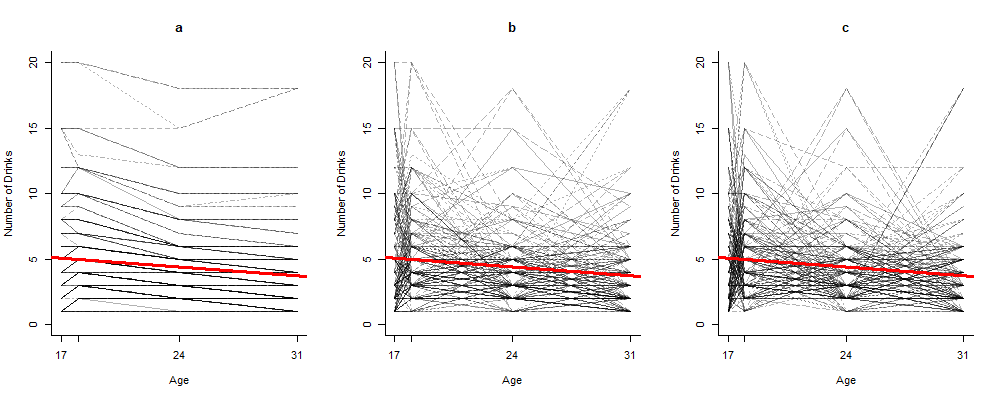
Note. Results of a Bayesian growth curve analysis of the average number of alcoholic drinks individuals reported drinking each time he/she drank alcohol. A permutation test showed no significant slope variation between individuals indicating a common downward trend across all individuals.
Significant fixed-effects for both the intercept and slope term were found for this model. At age 17, on average individuals reported drinking 5.06 alcoholic drinks with a standard deviation of 2.46. Each year after, individuals reported drinking 0.10 fewer drinks with a standard deviation of 0.26. When individuals reached age 31, on average they reported drinking 3.66 drinks. These results align with previous findings on alcohol consumption trajectories for the general population (Fillmore et al., 1991; Hartika et al., 1991). A permutation test found no meaningful interindividual differences in intraindividual change across time in drinking behavior for these individuals. This indicates that the slopes of individuals’ growth trajectories in alcohol use behavior did not reliably vary at the individual level, figure 2. That is, a single general downward trend is sufficient to describe how individuals drinking behaviors change across time, given that we can not reject the null-hypothesis that there is no variation between individuals in slope values. Although table 2 shows a 95% credible interval with positive values for the variance of the random slope term, this may be due to the boundary problem induced by utilizing gamma distributed priors used for the variance term. Additionally, the Effect:Error ratio for this data as assessed by our model was approximately 4:10. This indicates that our proposed method would have low statistical power in this case to pick up meaningful slope variation if it existed (as with using the DIC). As such these findings should be taken as only an example of our proposed method used on a real data set.
In order to facilitate the use of our proposed data permutation method, we have developed a web application for Bayesian analyses of unconditional growth curve models. See Figure 3 for the interface of the web application. This web application incorporates our proposed data permutation method and is made available for free at https://robertgm111.shinyapps.io/bayesiangrowthcurveapp/.
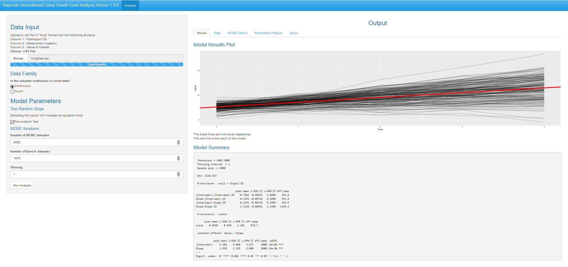
This web tool was made to give researchers a simple to use interface for conducting Bayesian analyses of unconditional growth curve models. A researcher interested in using this tool would need to have data in a 3-column long format with column 1 being participant ID, column 2 being measurement occasion, and column 3 being the quantity of interest. Researchers can then select if the outcome is continuous (modeled by an uninformative normal prior) or count (modeled by an uninformative Poisson). Additionally researchers may select to run the proposed permutation test for the existence of variable slopes at the cost of increased computation time. After specifying the number of MCMC samples, burn-in period, and thinning, a researcher can obtain parameter estimates under the “Model Summary” heading and a plot of the data with a fitted line based on the model under the “Model Results Plot” heading. Additional tabs in this web tool allow for data viewing, MCMC chain viewing and download, results of the proposed permutation test (if selected), and citing information in an “About” section. Missing data points are sampled from posterior distributions during the MCMC updating process.
The data permutation method shown in this article is a simple to use and widely applicable method for testing for the existence of interindividual differences in intraindividual change across time when these differences are modeled as gamma distributed variance components. Although itself not a Bayesian derived test, our method was able to perform on par with the DIC metric for most cases. Unlike more complicated methods such as DIC calculation and Bayes factors our permutation method requires little technical ability to implement, save for initial model specification. If a researcher is analysing data with a signal:noise ratio that is at least 1:1 then our method preforms just as well as common DIC comparison methods in terms of statistical power and outperforms DIC in terms of specificity. We do not believe this is an unreasonable ratio for many areas of psychological/behavioral sciences (Cooper & Findley, 1982; Wilson & Sherrell, 1993). Although other methods have been proposed for testing the existence of meaningful random slope variation, our proposed method is simple to use and we offer a direct software implementation (Saville & Herring, 2009).
Beyond ease of use, the permutation method displayed in this article represents an alternative method for model comparison in a Bayesian framework that is data driven. Many methods such as DIC and Bayes factors are manipulations of a model such that plausible models are pitted against one another so as to determine a model best fitting to a given data set. In such a model comparison framework, a given model is typically compared to a constrained version of itself (Kruschke, 2011; Spiegelhalter et al., 2002). These constrains represent a researcher’s qualities of interest, or unique hypotheses, regarding a specific data set. As opposed to constraining a specific parameter to test for the existence of a specific effect, our data driven method targets a quality if interest within the data itself. Instead of comparing a model with a given effect to a model without a given effect, our permutation method compares an estimated parameter (slope variation) from a given data set with the same parameter from both a modified data set in which this parameter has been destroyed and a second modified data set in which this parameter was amplified. That is, while model comparison asks ”Which model was more likely to generate this data?”, our proposed permutation method asks ”Is the parameter I am interested in modeling in this data different from data in which this parameter is just noise?”. Framing hypothesis testing in this manner is then a stepping stone to further data driven analyses in which a targeted permutation method is used to study a specific quality of interest.
Firstly, the support for our proposed method comes from our simulation study. Although we have attempted to model realistic circumstances given our specific random effects structure, our results can not be generalized outside of simulated parameterizations. Future work should focus on understanding the analytical properties of our test given that our test works on a bounded classification framework. This includes extending the results of this simulation to more time points, however we see no reason this method would not work on more than four time points.
Although simulation showed our method to have exceptional statistical power and specificity under conditions of relatively equal signal:noise ratios, there are still limitations to this method. One such limitation is that our proposed method showed inadequate statistical power of signal:noise ratios of 7:10 or less. Thus, our proposed method should not be used in situations in which variation in individual slopes is substantially less than error variance. In such a case DIC based model comparison is more appropriate. However, we believe that most longitudinal studies will easily be able to exceed this threshold, reducing the impact of this limitation. In situations in which significant covariance exists between intercept and slope values, our proposed method performs as well as DIC based model comparison. This is due to the necessity of the existence of slope variation prior to the existence of covariance between intercepts and slopes. In many realistic data sets, if significant slope exists then a significant covariance between intercept and slope is also likely to exist. This is due to ceiling effects, floor effects, regression to the mean, and other phenomenon common in behavioural data.
Our proposed method may also be limited in its usefulness beyond testing for significant slope variation. That is, our proposed method capitalizes on the fact that sorting data and shuffling data preserves intercept values and only changes error variance about slope estimates. Due to this capitalization, this permutation method is not applicable for testing for the existence of meaningful intercept variation and more research is needed to discover such a test. In practice however, researchers interested in longitudinal processes are generally more concerned with slope parameters as slope parameters represent change over time.
Additionally, this method only works for cases in which all participants have been sampled at the same discrete bins. That is, this method is not applicable for continuous sampling designs (Bolger & Laurenceau, 2013) In this case, alternative sorting and shuffling strategies must be employed so as to maintain the same structural changes int he data as would have occurred if the data was in discretely sampled bins at from the same time points. This also extends to cases of missing data. Missing data is common in longitudinal research and must be expected to occur more in studies over longer periods of time. In this case, multiple imputation may be used as a method for creating multiple possible tests using our algorithm. The most selected state (i.e., random effect or no random effect) across these imputations would then be chose as the best state to describe the data given the model.
One possible extension of the proposed data permutation method would be to test for nonlinear effects. Growth curve models are not limited to modeling solely linear growth, but may be extended to model curves of higher order polynomials (McArdle & Nesselroade, 2003). We do not see any reason for permutation testing to be ineffective for polynomial growth curve models, however this testing should still be conducted for purposes of understanding statistical power and specificity.
We also note the usefulness of plots of sorted data for understanding trajectories over time. Figures 1(a) and 2(a) show sorted data compared to original data in figures 1(b) and 2(b). Any linear trend is easier to visualize in the sorted data as opposed its associated original data. We attempted this same plotting method with non-linear effects as well and ac hived a similar ease of trend visualization, as sorting preserves intercept and slope values. Future research may specifically look at data sorting as a viable means of plotting data for model selection in growth curve analysis.
Other measures of distributional qualities besides the mean may also increase the power of our proposed method to detect significant slope variation across individuals. We conducted a relatively small simulation study testing the efficacy of using median estimates above mean estimates and obtained similar results to using means. Other metrics may prove to be more useful however, and should be tested in order to further refine our proposed data permutation method.
Another possible future direction would be to continue to create permutation tests targeting specific parameters of interest. According to Wolpert and Macready (1997), no single method for optimization of a problem is the best possible method for solving all problems. According to this No Free Lunch Theorem, the better a single optimizer gets at solving a specific problem, the worse it gets at solving all other problems. This suggests two things. Firstly, for every global method for optimizing a problem (e.g., DIC based model comparison), there exists a more targeted method that will yield a more optimal solution to a problem. Secondly, every problem may have its own ”best” solution. That is, every problem that is attempted to be optimized, may have its own best, and targeted, way to be optimized. While this second point implies that perhaps researchers should find targeted methodology for every possible effect in which they are interested, this would quickly spiral into many tests and would most likely create more confusion for individuals wishing to test specific effects.
Although targeted, our proposed method is easy to implement and solves the boundary problem for testing gamma/inverse gamma distributed random effects. This ease of implementation will allow more researchers to test for significant individual differences in intraindividual change. Additionally, our method offers one of the first steps for a paradigm shift of model comparison in a Bayesian framework. One where data is modified to destroy qualities of interest, as opposed to models being formed with/without qualities of interest. Indeed there may in fact be a hybrid form of these two methods that may prove more viable than either method in isolation. We hope our proposed permutation method spurs other researchers to consider data modifications for testing individual effects, leading to relatively uncomplicated methods that other researchers may use for testing whatever effects in which he/she is interested.
Baldwin, S. A., & Hoffmann, J. P. (2002). The Dynamics of Self-Esteem: A Growth-Curve Analysis. Journal of Youth and Adolescence, 31(2), 101–113. doi: https://doi.org/10.1023/A:1014065825598
Baltes, P. B., & Nesselroade, J. R. (1979). Longitudinal research in the study of behavior and development. Academic Press New York, NY.
Barr, D. J. (2013). Random effects structure for testing interactions in linear mixed-effects models. Frontiers in psychology, 4(December), 328. doi: https://doi.org/10.3389/fpsyg.2013.00328
Barr, D. J., Levy, R., Scheepers, C., & Tily, H. J. (2013). Random effects structure for confirmatory hypothesis testing: Keep it maximal. Journal of Memory and Language, 68(3), 255–278. doi: https://doi.org/10.1016/j.jml.2012.11.001
Bates, D. M., Kliegl, R., Vasishth, S., & Baayen, H. (2015). Parsimonious mixed models. arXiv preprint arXiv:1506.04967, 1–27. doi: https://doi.org/arXiv:1506.04967
Bayarri, M. J., & Berger, J. O. (2004). The interplay of bayesian and frequentist analysis. Statistical Science, 58–80. doi: https://doi.org/10.1214/088342304000000116
Bolger, N., & Laurenceau, J.-P. (2013). Intensive longitudinal methods: An introduction to diary and experience sampling research. Guilford Press.
Brooks, S. P., Giudici, P., & Philippe, A. (2003). Nonparametric convergence assessment for MCMC model selection. Journal of Computational and Graphical Statistics, 12(1), 1–22. doi: https://doi.org/10.1198/1061860031347
Cai, B., & Dunson, D. B. (2006). Bayesian covariance selection in generalized linear mixed models. Biometrics, 62(2), 446–457. doi: https://doi.org/10.1111/j.1541-0420.2005.00499.x
Carlin, B. P., & Chib, S. (1995). Bayesian Model Choice via Markov Chain Monte Carlo Methods. Journal of the Royal Statistical Society. Series B (Methodological), 57(3), 473–484. doi: https://doi.org/10.2307/2346151
Chen, Z., & Dunson, D. B. (2003). Random effects selection in linear mixed models. Biometrics, 59(4), 762–769.
Collingridge, D. S. (2013). A primer on quantitized data analysis and permutation testing. Journal of Mixed Methods Research, 7(1), 81–97. doi: https://doi.org/10.1177/1558689812454457
Cooper, H., & Findley, M. (1982). Expected Effect Sizes. Personality and Social Psychology Bulletin, 8(1), 168–173. doi: https://doi.org/10.1177/014616728281026
Efron, B. (1979). Bootstrap Methods: Another Look at the Jackknife. The Annals of Statistics, 7(1), 1–26. doi: https://doi.org/10.1214/aos/1176344552
Fan, Y., & Li, R. (2012). Variable selection in linear mixed effects models. Annals of Statistics, 40(4), 2043–2068. doi: https://doi.org/10.1214/12-AOS1028
Fearn, T. (1975). A Bayesian Approach to Growth Curves. Biometrika, 62(1), 89. doi: https://doi.org/10.2307/2334490
Fillmore, K. M., Hartika, E., Johnstone, B. M., Leino, E. V., Motoyoshi, M., & Temple, M. T. (1991). A meta-analysis of life course variation in drinking. British Journal of Addiction, 86(10), 1221–1268. doi: https://doi.org/10.1111/j.1360-0443.1991.tb01702.x
Gelman, A. (2006). Prior distributions for variance parameters in hierarchical models (Comment on Article by Browne and Draper). Bayesian Analysis, 1(3), 515–534. doi: https://doi.org/10.1214/06-BA117A
Gilks, W. R., Wang, C. C., Yvonnet, B., & Coursaget, P. (1993). Random-Effects Models for Longitudinal Data Using Gibbs Sampling. Biometrics, 49(2), 441. doi: https://doi.org/10.2307/2532557
Golland, P., & Fischl, B. (2003). Permutation tests for classification: towards statistical significance in image-based studies. In Biennial international conference on information processing in medical imaging (pp. 330–341).
Gomez-Baya, D., Mendoza, R., Paino, S., Sanchez, A., & Romero, N. (2016). Latent growth curve analysis of gender differences in response styles and depressive symptoms during mid-adolescence. Cognitive Therapy and Research, 1–15. doi: https://doi.org/10.1007/s10608-016-9822-9
Grimm, K. J., Ram, N., & Estabrook, R. (2016). Growth modeling: Structural equation and multilevel modeling approaches. Guilford Publications New York, NY.
Grimm, K. J., & Widaman, K. F. (2010). Residual structures in latent growth curve modeling. Structural Equation Modeling, 17(3), 424–442. doi: https://doi.org/10.1080/10705511.2010.489006
Gutman, L. M., Sameroff, A. J., & Cole, R. (2003). Academic growth curve trajectories from 1st grade to 12th grade: Effects of multiple social risk factors and preschool child factors. Developmental Psychology, 39(4), 777–790. doi: https://doi.org/10.1037/0012-1649.39.4.777
Hadfield, J. D. (2010). MCMCglmm: MCMC Methods for Multi-Response GLMMs in R. Journal of Statistical Software, 33(2), 1–22. doi: https://doi.org/10.1002/ana.22635
Hartika, E., Johnstone, B., Leino, E. V., Motoyoshi, M., Temple, M. T., & Fillmore, K. M. (1991). A meta-analysis of depressive symptomatology and alcohol consumption over time. British Journal of Addiction, 86(10), 1283–1298. doi: https://doi.org/10.1111/j.1360-0443.1991.tb01704.x
Hertzog, C., & Nesselroade, J. R. (2003). Assessing Psychological Change in Adulthood: An Overview of Methodological Issues. Psychology and Aging, 18(4), 639–657. doi: https://doi.org/10.1037/0882-7974.18.4.639
Hoijtink, H., van Kooten, P., & Hulsker, K. (2016). Bayes Factors Have Frequency Properties—This Should Not Be Ignored: A Rejoinder to Morey, Wagenmakers, and Rouder. Multivariate Behavioral Research, 51(1), 20–22. doi: https://doi.org/10.1080/00273171.2015.1071705
Kass, R. E., & Raftery, A. E. (1995). Bayes factors. Jounal of the american statistical association, 90(430), 773–795. doi: https://doi.org/10.1080/01621459.1995.10476572
Kruschke, J. K. (2011). Bayesian assessment of null values via parameter estimation and model comparison. Perspectives on Psychological Science, 6(3), 299–312. doi: https://doi.org/10.1177/1745691611406925
Lodewyckx, T., Kim, W., Lee, M. D., Tuerlinckx, F., Kuppens, P., & Wagenmakers, E. J. (2011). A tutorial on Bayes factor estimation with the product space method. Journal of Mathematical Psychology, 55(5), 331–347. doi: https://doi.org/10.1016/j.jmp.2011.06.001
Lunn, D., Jackson, C., Best, N., Spiegelhalter, D., & Thomas, A. (2012). The bugs book: A practical introduction to bayesian analysis. Chapman and Hall/CRC.
Lunn, D., Spiegelhalter, D., Thomas, A., & Best, N. (2009). The BUGS project: Evolution, critique and future directions. Statistics in Medicine, 28(25), 3049–3067. doi: https://doi.org/10.1002/sim.3680
Matuschek, H., Kliegl, R., Vasishth, S., Baayen, H., & Bates, D. (2017). Balancing Type I error and power in linear mixed models. Journal of Memory and Language, 94(2013), 305–315. doi: https://doi.org/10.1016/j.jml.2017.01.001
McArdle, J. J., & Nesselroade, J. R. (2003). Growth curve analysis in contemporary psychological research. In Handbook of psychology. John Wiley & Sons, Inc. doi: https://doi.org/10.1002/0471264385.wei0218
Morey, R. D., Wagenmakers, E. J., & Rouder, J. N. (2016). Calibrated Bayes Factors Should Not Be Used: A Reply to Hoijtink, van Kooten, and Hulsker. Multivariate Behavioral Research, 51(1), 11–19. doi: https://doi.org/10.1080/00273171.2015.1052710
Moulder, R. G., Boker, S. M., Ramseyer, F., & Tschacher, W. (2018). Determining synchrony between behavioral time series: An application of surrogate data generation for establishing falsifiable null-hypotheses. Psychological Methods. doi: https://doi.org/10.1037/met0000172
Oravecz, Z., & Muth, C. (2018). Fitting growth curve models in the Bayesian framework. Psychonomic Bulletin and Review, 25(1), 235–255. doi: https://doi.org/10.3758/s13423-017-1281-0
Peng, H., & Lu, Y. (2012). Model selection in linear mixed effect models. Journal of Multivariate Analysis, 109, 109–129. doi: https://doi.org/10.1016/j.jmva.2012.02.005
Pesarin, F., & Salmaso, L. (2010). The permutation testing approach: a review. Statistica, 70(4), 481–509. doi: https://doi.org/10.6092/issn.1973-2201/3599
Piironen, J., & Vehtari, A. (2017). Comparison of bayesian predictive methods for model selection. Statistics and Computing, 27(3), 711–735. doi: https://doi.org/10.1007/s11222-016-9649-y
R Core Team. (2013). R: A language and environment for statistical computing [Computer software manual]. Vienna, Austria. Retrieved from http://www.R-project.org/
Roberts, B. W., Walton, K. E., & Viechtbauer, W. (2006). Patterns of mean-level change in personality traits across the life course: a meta-analysis of longitudinal studies. Psychological bulletin, 132(1), 1. doi: https://doi.org/10.1037/0033-2909.132.1.1
Rouder, J. N., & Morey, R. D. (2012). Default Bayes Factors for Model Selection in Regression. Multivariate Behavioral Research, 47(6), 877–903. doi: https://doi.org/10.1080/00273171.2012.734737
Saville, B. R., & Herring, A. H. (2009). Testing Random Effects in the Linear Mixed Model Using Approximate Bayes Factors. Biometrics, 65(2), 369–376. doi: https://doi.org/10.1111/j.1541-0420.2008.01107.x
Shedler, J., & Block, J. (1990). Adolescent drug use and psychological health: A longitudinal inquiry. American psychologist, 45(5), 612. doi: https://doi.org/10.1037//0003-066X.45.5.612
Silver, R. C., Holman, E. A., McIntosh, D. N., Poulin, M., & Gil-Rivas, V. (2002). Nationwide longitudinal study of psychological responses to september 11. Jama, 288(10), 1235–1244. doi: https://doi.org/10.1001/jama.288.10.1235
Spiegelhalter, D. J., Best, N. G., & Carlin, B. P. (1998). Bayesian deviance, the effective number of parameters , and the comparison of arbitrarily complex models. Technical Report, MRC Biostatistics Unit, Cambridge, UK.
Spiegelhalter, D. J., Best, N. G., Carlin, B. P., & van der Linde, A. (2002). Bayesian Measures of Model Complexity anf Fit. Journal of the Royal Statistical Society Series B (Statistical Methodology), 64(4), 583–639. doi: https://doi.org/10.1111/1467-9868.00353
Spiegelhalter, D. J., et al. (2014). The deviance information criterion: 12 years on (with discussion). Journal of the Royal Statistical Society: Series B, 64, 485–493. doi: https://doi.org/10.1111/rssb.12062
Stefan, A. M., Gronau, Q. F., Schönbrodt, F. D., & Wagenmakers, E.-J. (2019). A tutorial on bayes factor design analysis using an informed prior. Behavior research methods, 51(3), 1042–1058. doi: https://doi.org/10.3758/s13428-018-01189-8
Stram, D. O., & Lee, J. W. (1994, dec). Variance Components Testing in the Longitudinal Mixed Effects Model. Biometrics, 50(4), 1171. doi: https://doi.org/10.2307/2533455
Sturtz, S., Ligges, U., & Gelman, A. (2005). R2OpenBUGS: A Package for Running OpenBUGS from R. Journal of Statistical Software, 12(3), 1–16. doi: https://doi.org/10.18637/jss.v012.i03
Theiler, J., Eubank, S., Longtin, A., Galdrikian, B., & Farmer, J. D. (1992). Testing for nonlinarity in time series: the method of surrogate data. Physica D, 58(1-4), 77–94. doi: https://doi.org/10.1016/0167-2789(92)90102-S
Vaida, F., & Blanchard, S. (2005). Conditional Akaike information for mixed-effects models. Biometrika, 92(2), 351–370. doi: https://doi.org/10.1093/biomet/92.2.351
Ward, E. J. (2008). A review and comparison of four commonly used Bayesian and maximum likelihood model selection tools. Ecological Modelling, 211(1-2), 1–10. doi: https://doi.org/10.1016/j.ecolmodel.2007.10.030
Wilson, E. J., & Sherrell, D. L. (1993). Source Effects in Communication and Persuasion Research:. Journal of the Academy of Marketing Science, 21(2), 101. doi: https://doi.org/10.1177/009207039302100202
Wolpert, D., & Macready, W. (1997, apr). No free lunch theorems for optimization. IEEE Transactions on Evolutionary Computation, 1(1), 67–82. Retrieved from http://ieeexplore.ieee.org/document/585893/ doi: https://doi.org/10.1109/4235.585893
Zhang, Z. (2016). Modeling error distributions of growth curve models through Bayesian methods. Behavior Research Methods, 48(2), 427–444. doi: https://doi.org/10.3758/s13428-015-0589-9
Zhang, Z., Hamagami, F., Wang, L., Nesselroade, J. R., & Grimm, K. J. (2007). Bayesian analysis of longitudinal data using growth curve models. International Journal of Behavioral Development, 31(4), 374–383. doi: https://doi.org/10.1177/0165025407077764